FIFA Women’s World Ranking and goal difference in Elo ratings.

The FIFA rankings for women’s national teams use a quite different methodology than the one used in ranking men’s national teams. The Women’s World Ranking (WWR) is based on the Elo rating system I wrote about in the previous post. The details for the men’s ranking can be found here, and the details the women’s ranking can be found here.

One thing that makes the WWR interesting is how goal differences are accounted for in the ratings. This is not something found in the ordinary chess-based Elo ratings. The method used in WWR is to let the ‘winning percentage’ change depending on two things: Goal difference and the number of goals the loosing team scored. This is in contrast to the original Elo ratings where the winning team wins 100% and the loosing team wins 0% (a draw is 50%). In WWR a team can never win 100%, the most it can win is 99%. This is the case when the goal difference is more than 6 and the loosing team haven’t scored any goals. The table below is from the pdf file linked to above and shows how many percent the loosing team win.

wwrtable

One strange thing about this table is the column for goal difference 0, implying a draw. I am guessing this is an error since it means that the winning percentage for the loosing team will be greater than the winning team. In the paper I mentioned in my last post where a number of different rating methods were compared (The predictive power of ranking systems in association football by J. Laset et. al), it was assumed that draw would yield both teams 50%, as in the original Elo-ratings. That paper also showed that the Women’s World Ranking was among the rating systems with best prediction.

Here is a plot showing the win percentage when the loosing team has scored 0 and 5 goals. We can see that there is not much gained for the loosing team to score one extra goal (assuming the goal difference stays the same, which of course is dubious), and most of the gain in winning percentage is when a team scores a goal such that the stance goes from a draw to a win.

WWRwinpercantage_nontransparent

The table above only goes up to 5 goals for the loosing team, but for the sake of implementation it is easy to generalize the rule about how much the loosing team gains by scoring an additional goal (with the goal difference is the same). For example will the loosing team gain 0.9 extra winning percentage points when the goal difference is 2. Similarly the gain is 0.6 percentage points when the goal difference is 5.

Below is a R function to compute the win percentage for football matches. It takes as input two vectors with the number of goals scored by the two opponents and returns a vector of win percentages (a number between 0 and 1) for the first team.

winPercentageWWR <- function(team1Goals, team2Goals){
  #calculates the win percentage for team 1.

  stopifnot(length(team1Goals) == length(team2Goals))
  
  perc <- c(0.01, 0.02, 0.03, 0.04, 0.08, 0.15, 0.50, 0.85, 0.92, 0.96, 0.97, 0.98, 0.99)
  add <- c(0, 0.01, 0.009, 0.008, 0.007, 0.006, 0.005)
  
  goalDifferences <- (team1Goals - team2Goals)
  goalDifferences[goalDifferences < -6] <- -6
  goalDifferences[goalDifferences > 6] <- 6

  team1WinPercentage <- numeric(length=length(goalDifferences))

  for (idx in 1:length(goalDifferences)){

    team1WinPercentage[idx] <- perc[goalDifferences[idx]+7] -  
      sign(goalDifferences[idx])*min(team1Goals[idx], team2Goals[idx])*add[abs(goalDifferences[idx])+1]
  }
  return(team1WinPercentage) 
}

Elo ratings in football

I have previously written about some statistical methods for rating football teams and to predict the result of future matches. One was the last squares method and another was the Poisson regression method. None of these methods make good enough predictions. One problem with them is that they don’t incorporate a time perspective. Matches played a year ago is given equal importance as the most recent one. This could however be incorporated by weighing the the older matches less than newer matches. One other problem that I mentioned in the second post about Poisson regression is that teams are treated as categoricals which makes it hard to model the fact that a team’s ability changes over time.

One different kind of method that has been employed a lot in the recent years is the Elo rating system, which were originally developed for rating chess players. The method is rather simple, but I will not explain it in detail here since there are many good explanations of it elsewhere. Wikipedia has a very thorough coverage. The basic principle is that the difference in ratings between the two opposing teams provide a prediction for the result each game. The rating is then updated based on how the teams perform. If a team performs better than expected the rating increases, if they perform worse than expected the rating decrease. How much the rating changes depends on an update factor (often referred to as the K-factor).

Chess and football are of course different in many ways so the method for rating chess players is not directly suitable for rating football teams. The relative simplicity of the Elo system makes it easy to tweak and adjust to better fit football by incorporating things like home field advantage and goal difference. There are many sites around the Internet who provide different variants of Elo ratings, like the World Football Elo Ratings for national teams and Club Elo and Euro Club Index for club teams. FIFA even uses its own Elo system in its Womans World Ranking.

There has even been some research into different football rating systems. A paper titled The predictive power of ranking systems in association football (pdf) by Jan Lasek and others compared different rating systems. Their conclusion was that the different Elo type systems in general were better at predicting match outcomes than other types of rating systems.

I figured I wanted to implement a simple Elo rating system for rating football teams. There is already a package in R, PlayerRatings, which implements several different rating systems based on Elo. In my simple implementation there is no adjustment for goal difference, but I have support for home field advantage. All teams start with an initial rating of 1500. Here is what I got when I calculated the ratings for Premier League in November 2012 based on data going back to 1993. I used an update factor 24 without any home field advantage. There is no particular reason for this as I did this mostly as a proof of concept.

  Rating (November 2012)
Man United 1807
Man City 1767
Chelsea 1696
Arsenal 1658
Tottenham 1645
Everton 1640
Newcastle 1613
Fulham 1591
Liverpool 1567
West Brom 1562
Leeds 1552
Wigan 1543
Swansea 1526
Sunderland 1524
Stoke 1521
Middlesboro 1516
Norwich 1509
Aston Villa 1498
West Ham 1494
Birmingham 1493
Blackpool 1483
Ipswich 1481
Bolton 1479
Charlton 1470
Sheffield United 1458
Blackburn 1450
Reading 1448
Sheffield Weds 1447
Coventry 1447
Middlesbrough 1443
QPR 1440
Barnsley 1439
Portsmouth 1438
Southampton 1437
Oldham 1436
Crystal Palace 1433
Leicester 1433
Nott’m Forest 1430
Hull 1422
Burnley 1418
Wolves 1414
Wimbledon 1413
Watford 1411
Bradford 1406
Swindon 1404
Derby 1297

The table seems reasonable I think except for a couple of things. There is a problem related to relegation and promotion. Since I have used data back to 1993 every team who has played in the Premier League is given a rating. If a team is relegated to the Championship, their rating will no longer be updated. We can see that this creates some strange results. Take the two lowest rated teams for example. Derby has not been in the Premier League since the 2007-2008 season. Swindon, which is rated about 100 points higher than Derby, has not played in the Premier League since 1993-1994 season! Swindon now play in the fourth level of the English league system. So the ratings for the teams not in the Premier League should be considered invalid.

Relegation and promotion also creates a problem with inflated ratings. The Elo system is created so that the total number of points in the league should be constant. When a team is promoted they start with an initial rating of 1500, and if they later gets relegated they will probably have lost some of those points to the other teams in the league. In fact, we see that many of the teams with ratings less than 1500 no longer plays in the Premier League. The points they have lost are still in present in the league even though the team isn’t. This means that over time the average ratings of the teams in the league will increase.

The code I have written takes a data frame as input and works “out of the box” with data from football-data.co.uk. If you are going to use it yourself you have to make sure the data is sorted by date as the rating function just loops from top to bottom.

Here is how you can use it:

dta <- read.csv("yourdata.csv")
elo <- eloRating(data=dta)
print(elo)

And here is the code:


eloRating <- function(home="HomeTeam", away="AwayTeam", homeGoals="FTHG",
                      awayGoals="FTAG", data, kfactor=24, initialRating=1500,
                      homeAdvantage=0){
  
  #Make a list to hold ratings for all teams
  all.teams <- levels(as.factor(union(levels(as.factor(data[[home]])),
                                      levels(as.factor(data[[away]])))))
  
  ratings <- as.list(rep(initialRating, times=length(all.teams)))
  names(ratings) <- all.teams

  #Loop trough data and update ratings
  for (idx in 1:dim(data)[1]){
  
    #get current ratings
    homeTeamName <- data[[home]][idx]
    awayTeamName <- data[[away]][idx]
    homeTeamRating <- as.numeric(ratings[homeTeamName]) + homeAdvantage
    awayTeamRating <- as.numeric(ratings[awayTeamName])
    
    #calculate expected outcome 
    expectedHome <- 1 / (1 + 10^((awayTeamRating - homeTeamRating)/400))
    expectedAway <- 1 - expectedHome
    
    #Observed outcome
    goalDiff <- data[[homeGoals]][idx] - data[[awayGoals]][idx]
    if (goalDiff == 0){
      resultHome <- 0.5
      resultAway <- 0.5
    }
    else if (goalDiff < 0){
      resultHome <- 0
      resultAway <- 1
    }
    else if (goalDiff > 0){
      resultHome <- 1
      resultAway <- 0
    }
    
    #update ratings
    ratings[homeTeamName] <- as.numeric(ratings[homeTeamName]) + kfactor*(resultHome - expectedHome)
    ratings[awayTeamName] <- as.numeric(ratings[awayTeamName]) + kfactor*(resultAway - expectedAway)
  }
  
  #prepare output
  ratingsOut <- as.numeric(ratings)
  names(ratingsOut) <- names(ratings)
  ratingsOut <- sort(ratingsOut, decreasing=TRUE)

  return(ratingsOut) 
}

Predicting football results with Poisson regression pt. 2

In part 1 I wrote about the basics of the Poisson regression model for predicting football results, and briefly mentioned how our data should look like. In this part I will look at how we can fit the model and calculate probabilities for the different match outcomes. I will also discuss some problems with the model, and hint at a few improvements.

Fitting the model with R
When we have the data in an appropriate format we can fit the model. R has a built in function glm() that can fit Poisson regression models. The code for loading the data, fitting the model and getting the summary is simple:

#load data
yrdta <- read.csv(“yourdata.csv”)

#fit model and get a summary
model <- glm(Goals ~ Home + Team + Opponent, family=poisson(link=log), data=yrdta)
summary(model)

The summary function for fitting the model with data from Premier League 2011-2012 season gives us this (I have removed portions of it for space reasons):

(Edit September 2014: There was some errors in the estimates in the original version of this post. This was because I made some mistakes when I formated the data as described in part one. Thanks to Derek in the comments for pointing this out. )

Coefficients:
                    Estimate Std. Error z value Pr(>|z|)    
(Intercept)          0.45900    0.19029   2.412 0.015859 *  
Home                 0.26801    0.06181   4.336 1.45e-05 ***
TeamAston Villa     -0.69103    0.20159  -3.428 0.000608 ***
TeamBlackburn       -0.40518    0.18568  -2.182 0.029094 *  
TeamBolton          -0.44891    0.18810  -2.387 0.017003 *  
TeamChelsea         -0.13312    0.17027  -0.782 0.434338    
TeamEverton         -0.40202    0.18331  -2.193 0.028294 *  
TeamFulham          -0.43216    0.18560  -2.328 0.019886 *
-----
OpponentSunderland  -0.09215    0.20558  -0.448 0.653968    
OpponentSwansea      0.01026    0.20033   0.051 0.959135    
OpponentTottenham   -0.18682    0.21199  -0.881 0.378161    
OpponentWest Brom    0.03071    0.19939   0.154 0.877607    
OpponentWigan        0.20406    0.19145   1.066 0.286476    
OpponentWolves       0.48246    0.18088   2.667 0.007646 ** 
---
Signif. codes:  0 ‘***’ 0.001 ‘**’ 0.01 ‘*’ 0.05 ‘.’ 0.1 ‘ ’ 1

The Estimate column is the most interesting one. We see that the overall mean is e0.49 = 1.63 and that the home advantage is e0.26 = 1.30 (remember that we actually estimate the logarithm of the expectation, therefore we need to exponentiate the coefficients to get interpretable numbers). If we want to predict the results of a match between Aston Villa at home against Sunderland we could plug the estimates into our formula, or use the predict() function in R. We need to do this twice, one time to predict the number of goals Aston Villa is expected to score, and one time for Sunderland.

#aston villa
predict(model, data.frame(Home=1, Team="Aston Villa", Opponent="Sunderland"), type="response")
# 0.9453705 

#for sunderland. note that Home=0.
predict(model, data.frame(Home=0, Team="Sunderland", Opponent="Aston Villa"), type="response")
# 0.999 

We see that Aston Villa is expected to score on average 0.945 goals, while Sunderland is expected to score on average 0.999 goals. We can plot the probabilities for the different number of goals against each other:

AstonVillaSunderland1

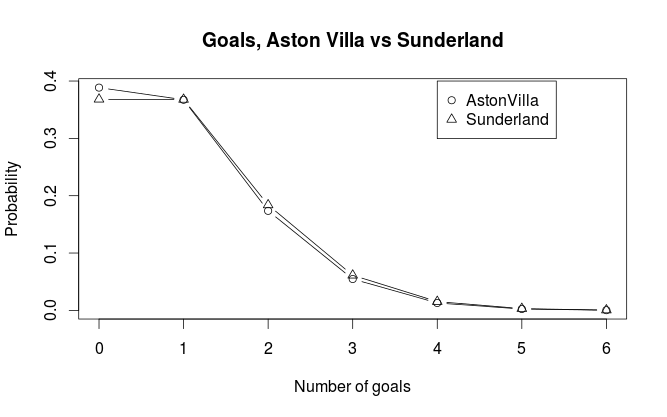
We can see that Aston Villa has just a bit higher probability for scoring not goals than Sunderland. Sunderland has also just a tiny bit higher probablity for most other number of goals. Both teams have about the same probability of scoring exactly one goal. In general the pattern we see in the plot is consistent with what we would expect considering the expected number of goals.

Match result probabilities
Now that we have our expected number of goals for the two opponents in a match, we can calculate the probabilities for either home win (H), draw (D) and away win (A). But before we continue, there is an assumption in our model that needs to be discussed, namely the assumption that the goals scored by the two teams are independent. This may not be obvious since surely we have included information about who plays against who when we predict the number of goals for each team. But remember that each match is included twice in our data set, and the way the regression method works, each observation are assumed to be independent from the others. We’ll see later that this can cause some problems.

The most obvious way calculate the probabilities of the three outcomes is perhaps to look at goal differences. If we can calculate the probabilities for goal differences (home goals minus away goals) of exactly 0, less than 0, and greater than 0, we get the probabilities we are looking for. I will explain two ways of doing this, both yielding the same result (in theory at least): By using the Skellam distribution and by simulation.

Skellam distribution
The Skellam distribution is the probability distribution of the difference of two independent Poisson distributed variables, in other words, the probability distribution for the goal difference. R does not support it natively, but the VGAM package does. For our example the distribution looks like this:
AstonVillaSunderland2
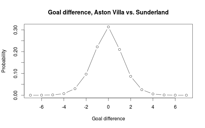
If we do the calculations we get the probabilities for home win, draw, away win to be 0.329, 0.314, 0.357 respectively.

#Away
sum(dskellam(-100:-1, predictHome, predictAway)) #0.3574468
#Home
sum(dskellam(1:100, predictHome, predictAway)) #0.3289164
#Draw
sum(dskellam(0, predictHome, predictAway)) #0.3136368

Simulation
The second method we can use is simulation. We simulate a number of matches (10000 in our case) by having the computer draw random numbers from the two Poisson distributions and look at the differences. We get the probabilities for the different outcomes by calculating the proportion of different goal differences. The independence assumption makes this easy since we can simulate the number of goals for each team independently of each other.

 set.seed(915706074)
nsim <- 10000
homeGoalsSim <- rpois(nsim, predictHome) 
awayGoalsSim <- rpois(nsim, predictAway)
goalDiffSim <- homeGoalsSim - awayGoalsSim
#Home
sum(goalDiffSim > 0) / nsim #0.3275
#Draw
sum(goalDiffSim == 0) / nsim # 0.3197
#Away
sum(goalDiffSim < 0) / nsim #0.3528

The results differ a tiny bit from what we got from using the Skellam distribution. It is still accurate enough to not cause any big practical problems.

How good is the model at predicting match outcomes?
The Poisson regression model is not considered to be among the best models for predicting football results. It is especially poor at predicting draws. Even when the two teams are expected to score the same number of goals it rarely manages to assign the highest probability for a draw. In one attempt I used Premier League data from the last half of one season and the first half of the next season to predict the second half of that season (without refitting the model after each match day). It assigned highest probability to the right outcome in 50% of the matches, but never once predicted a draw.

Lets see at some other problems with the model and suggest some improvements.

One major problem I see with the model is that the predictor variables are categorical. This is a constraint that makes inefficient use of the available data since we get rather few data points per parameter (i.e per team). The model does for example not understand teams are more like each other than others and instead view each team in isolation. There has been some attempts at using Bayesian methods to incorporate information on which teams are better and which are poorer. Se for example this blog. If the teams instead could be reduced to numbers (by using some sort of rating system) we would get fewer parameters to estimate. We could then also incorporate an interaction term, something that is almost impossible with the categorical predictor variables we have. The interaction term in this case would be the effect of a team under or over estimating its opponent.

(As an aside, we could in fact interpret the coefficients in our model as a form of rating of a teams offensive and defensive strength)

Another way the model can be improved is to incorporate a time aspect. The most obvious way to do this is perhaps to weights to the matches such that more recent matches are more important than matches far back in time.

A further improvement would be to look at the level of different players, and not at a team as a whole. For example will a team with many injured players in a match most likely perform poorer than what you would expect. One could use weights to down weight the contribution of matches where this is a problem. A much more powerful idea would be to combine data on match lineup with a rating system for players. This could be used to infer a rating for the whole team in a specific match. In addition to correct for injured players it would also account for new players on a team and players leaving a team. The biggest problem with this approach is lack of available data in a format that is easy to handle.

I don’t think any of the improvements I have discussed here will solve the problem of predicting draws since it originates in the independent Poisson assumption, although I think they could improve predictions in general. To counter the problem of predicting draws I think a very different model would have to be used. I would also like to mention that the improvements I have suggested here are rather general, and could be incorporated in many other prediction models.

Predicting football results with Poisson regression pt. 1

I have been meaning to write about my take on using Poisson regression to predict football results for a while, so here we go. Poisson regression is one of the earliest statistical methods used for predicting football results. The goal here is to use available data to to say something about how many goals a team is expected to score and from that calculate the probabilities for different match outcomes.

The Poisson distribution
The Poisson distribution is a probability distribution that can be used to model data that can be counted (i.e something that can happen 0, 1, 2, 3, … times). If we know the number of times something is expected to happen, we can find the probabilities that it happens any number of times. For example if we know something is expected to happen 4 times, we can calculate the probabilities that it happens 0, 1, 2, … times.

It turns out that the number of goals a team scores in a football match are approximately Poisson distributed. This means we have a method of assigning probabilities to the number of goals in a match and from this we can find probabilities for different match results. Note that I write that goals are approximately Poisson. The Poisson distribution does not always perfectly describe the number of goals in a match. It sometimes over or under estimates the number of goals, and some football leagues seems fit the Poisson distribution better than others. Anyway, the Poisson distribution seems to be an OK approximation.

The regression model
To be able to find the probabilities for different number of goals we need to find the expected number of goals L (It is customary to denote the expectation in a Poisson distribution by the Greek letter lambda, but WordPress seem to have problems with greek letters so i call i L instead). This is where the regression method comes in. With regression we can estimate lambda conditioned on certain variables. The most obvious variable to look at is which team is playing. Manchester United obviously makes more goals than Wigan. The second thing we want to take into account is who the opponent is. Some teams are expected to concede fewer goals, while others are expected to let in more goals. The third thing we want to take into account is home field advantage.

Written in the language of regression models this becomes

log(L) = mu + home + teami + opponentj

The mu is the overall mean number of goals. The home is the effect on number of goals a team has by playing at home. Teami is the effect of team number i, opponentj is the effect of team j.

(Note: Some descriptions of the Poisson regression model on football data uses the terms offensive and defensive strength to describe what I have called team and opponent. The reason I prefer the terms I use here is because it makes it a bit easier to understand later when we look at the data set.)

The logarithm on the left hand side is called the link function. I will not dwell much on what a link function is, but the short story is that they ensure that the parameter we try to estimate don’t fall outside its domain. In this case it ensures us that we never get negative expected number of goals.

Data
In my example I will use data from football-data.co.uk. What data you would want to use is up to yourself. Typically you could choose to use data from the last year or the least season, but that is totally up to you to decide.

Each of the terms on the right hand side of the equation (except for mu) corresponds to a columns in a table, so we need to fix our data a bit before we proceed with fitting the model. Each match is essentially two observations, one for how many goals the home team scores, the second how many the away team scores. Basically, each match need two rows in our data set, not just one.

Doing the fix is an easy thing to do in excel or Libre Office Calc. We take the data rows (i.e. the matches) we want to use and duplicate them. Then we need to switch the away team and away goals columns so they become the same as the home team column. We also need a column to indicate the home team. Here is an example on how it will look like:

In the next part I will fit the actual model, calculate probabilities and describe how we can make predictions using R.

‘Synonymous’ factor levels in R

When I work with data from different sources, they are often inconsistent in ways they specify categorical variables. One example is country names. There are many ways the name of a country can be specified, and even if there are international standards, different organizations like to do it their way. North Korea, for example, may sometimes be written as just as ‘North Korea’, but other sources may call it ‘Korea DPR’.

This of course leads to complications when we want to combine data from different sources. What could be a trivial lookup in two different dataframes in R becomes a real hassle. One solution I have come up with is to make a .csv file with different names from different sources, and then load it into R and use it to ‘translate’ the factor levels from one source to the way the levels are represented in the other. Based on a method for renaming levels with regular expressions from Winston Chang’s Cookbook for R, I made a function for renaming several levels in a dataframe at once. The part about using a .csv file is not the important thing here, it is just a more convenient way of storing the information needed.

The function takes four arguments. dat is a dataframe that contains the factors that is to be renamed. vars is the variables to rename. from and to specifies what to rename from and what to rename to. The function returns a dataframe.

renameLevels <- function(dat, vars, from, to){
  for (v in vars){
    ptrns <- paste("^", from, "$", sep="") 
    for (lvl in 1:length(ptrns)){
      levels(dat[, v]) <- sub(ptrns[lvl], to[lvl], levels(dat[, v]))
    }
  }
  return(dat)
}

A small example:

#data to be translated
var <- factor(c("b", "a", "c", "a", "d", "a", "e", "b"))
var2 <- factor(c("b", "b", "b", "b", "b", "a", "e", "b"))
data <- data.frame(var, var2)
#> data
#  var var2
#1   b    b
#2   a    b
#3   c    b
#4   a    b
#5   d    b
#6   a    a
#7   e    e
#8   b    b

#translate from roman to greek letters
roman <- c("a", "b", "c", "d", "e")
greek <- c("alpha", "beta", "gamma", "delta", "epsilon")

data2 <- renameLevels(data, c("var", "var2"), roman, greek)
#> data2
#      var    var2
#1    beta    beta
#2   alpha    beta
#3   gamma    beta
#4   alpha    beta
#5   delta    beta
#6   alpha   alpha
#7 epsilon epsilon
#8    beta    beta

Least squares rating of football teams

The Wikipedia article Statistical association football predictions mentions a method for least squares rating of football teams. The article does not give any source for this, but I found what I think may be the origin of this method. It appears to be from an undergrad thesis titled Statistical Models Applied to the Rating of Sports Teams by Kenneth Massey. It is not on football in particular, but on sports in general where two teams compete for points. A link to the thesis can be found here.

The basic method as described in Massey’s paper and the Wikipedia article is to use a n*k design matrix A where each of the k columns represents one team, and each of the n rows represents a match. In each match (or row) the home team is indicated by 1, and the away team by -1. Then we have a vector y indicating goal differences in each match, with respect to the home team (i.e. positive values for home wins, negative for away wins). Then the least squares solution to the system Ax = y is found, with the x vector now containing the rating values for each team.

When it comes to interpretation, the difference in least squares estimate for the rating of two teams can be seen as the expected goal difference between the teams in a game. The individual rating can be seen as how many goals a teams scores compared to the overall average.

Massey’s paper also discusses some extensions to this simple model that is not mentioned in the Wikipedia article. The most obvious is incorporation of home field advantage, but there is also a section on splitting the teams’ performances into offensive and defensive components. I am not going to go into these extensions here, you can read more about them i Massey’s paper, along with some other rating systems that are also discussed. What I will do, is to take a closer look at the simple least squares rating and compare it to the ordinary three points for a win rating used to determine the league winner.

I used the function I made earlier to compute the points for the 2011-2012 Premier League season, then I computed the least squares rating. Here you can see the result:

  PTS LSR LSRrank RankDiff
Man City 89 1.600 1 0
Man United 89 1.400 2 0
Arsenal 70 0.625 3 0
Tottenham 69 0.625 4 0
Newcastle 65 0.125 8 3
Chelsea 64 0.475 5 -1
Everton 56 0.250 6 -1
Liverpool 52 0.175 7 -1
Fulham 52 -0.075 10 1
West Brom 47 -0.175 12 2
Swansea 47 -0.175 11 0
Norwich 47 -0.350 13 1
Sunderland 45 -0.025 9 -4
Stoke 45 -0.425 15 1
Wigan 43 -0.500 16 1
Aston Villa 38 -0.400 14 -2
QPR 37 -0.575 17 0
Bolton 36 -0.775 19 1
Blackburn 31 -0.750 18 -1
Wolves 25 -1.050 20 0

It looks like the Least squares approach gives similar results as the standard points system. It differentiates between the two top teams, Manchester City and Manchester United, even if they have the same number of points. This is perhaps not so surprising since City won the league because of greater goal difference than United, and this is what the least squares rating is based on. Another, perhaps more surprising thing is how relatively low least squares rating Newcastle has, compared to the other teams with approximately same number of points. If ranked according to the least squares rating, Newcastle should have been below Liverpool, instead they are three places above. This hints at Newcastle being better at winning, but with few goals, and Liverpool winning fewer times, but when they win, they win with more goals. We can also see that Sunderland comes poor out in the least squares rating, dropping four places.

If we now plot the number of points to the least squares rating we see that the two methods generally gives similar results. This is perhaps not so surprising, and despite some disparities like the ones I pointed out, there are no obvious outliers. I also calculated the correlation coefficient, 0.978, and I was actually a bit surprised of how big it was.

Very accurate music reviews are perhaps not so useful

Back in august i downloaded all album reviews from pitchfork.com, a hip music website mainly dealing with genres such as rock, electronica, experimental music, jazz etc. In addition to a written review, each reviewed album is given a score by the reviewer from 0.0 to 10.0, to one decimal accuracy. In other words, a reviewed album is graded on a 101 point scale. But does it make sense to have such an accurate grading scale? Is it really any substantial difference between two records with a 0.1 difference in score? Listening to music is a qualitative experience, and no matter how professional the reviewer is, a record review is always a subjective analysis influenced by the reviewers taste, mood and preconceptions. To quantify musical quality on a single scale is therefore a hard, if not impossible, feat. Still, new music releases is routinely reviewed and graded in the media, but i don’t know of anyone having a grading system to the accuracy that Pitchfork does. Usually there is a 0 to 5 or 0 to 10 scale, perhaps to the accuracy of a half. There are sites like Metacritc and Rotten Tomatoes (for film reviews) that has a similar accuracy to their reviews, but they are both based on reviews collected from many sources. In the case of Pitchfork, there is usually just one reviewer (with a few reviews credited to two or more people). As far as i know pitchfork has no guidelines on how to interpret the score or what criteria they use to set the score and it may just be up to the reviewer to figure out what to put in the score.

Anyway, I extracted the information from the reviews i downloaded and put it into a .csv file. This gave me data on 13330 reviews which i then loaded into R for some plotting with ggplot2. Lets look at some graphs to see how the scores are distributed and try to find something interesting. First we have a regular histogram:

When I first saw it I was not expect the distribution to be so right skewed. I expected the top to be around maybe 5 or 6. I calculated the mean and median which are 6.96 and 7.2, respectively. Lets look at a bar plot, where each bar corresponds to a specific score.

Now this is interesting. We can clearly see four spikes around the top, some scores are clearly more popular than others. ggplot2 clutters the ticks on the x-axis so it is difficult to see exactly which scores it is (this seems to be a regular problem with ggplot2, event the examples in the official documentation suffers from this) Anyway, I found out that the most popular scores are 7.5 (620 records), 7.0 (614 records), 7.8 (611 records) and 8.0 (594 records). Together, 18.3% of the reviewed records has been given one of these four scores. From this it seems to be some sort of bias towards round or ‘half round’ numbers. I guess we humans have some sort of subconscious preference for these kinds of numbers. If we now look closer at the right end of the plot, we see the same phenomena:

The 10.0 ‘perfect’ score is way more used than the scores just below it. So it appears to be harder to make a ‘near perfect’ album than a perfect one, which is kind of strange. If I were to draw some conclusion after looking at these charts, it would be that a 101 point scale is too accurate to be useful for distinguish between albums that differ little in their numeric scores. I also wonder if this phenomenon can be found in other situations where people are asked to grade something on a scale with similar accuracy.

Looking at monthly distribution of births in Norway

A news story earlier this week reported an increased number of births during the summer months in Norway. According to the story the peak in births used to be in the spring months, nine months after summer vacation, but is now during the summer. The midwifes thinks this change is because of the rules for granting a place in preschool day care. Children born before september 1st are legally entitlet to a place in day care.

Anyway i decided to try to visualize this. I found some data at the Statistics Norway website, loaded it into R, cleaned it, restructured it etc. and made this animation with ggplot2 showing the monthly distribution of births from year 2000 to 2011. I decided to include data for the years before 2005 since that is when the current left wing coalition took office and they had a program for universal access to day care. It is hard to spot a definite trend, but the graph for 2011 shows a clear top in the summer months. It will be interesting to see if this becomes clearer the next couple of years. Also, if this becomes a continuing trend, it would be interesting to look at surveys in family planning and see if there has been more of it the last couple of years.

The birthIndex on the y-axis is not the precise number of births for a given month, but is corrected for the number of days in the month. This makes the different months comparable.

R functions for soccer league tables and result matrix

Here are three R functions i wrote to calculate ranking tables in soccer leagues based on the result of played matches. The functions are made for ordinary leagues where each team play every other team twice, one time at the home field, the other at the opposing teams home field, but the match.result() and league.table() function can be used on more general data.

The first function, match.results() just computes the outcome of a match (Home, Draw or Away, i.e “H”, “D” or “A”) based on number of goals scored, and is used by the other two functions.

> res <- match.results(c(1,2,1,2,3,1,0,5), c(0,1,2,0,3,0,4,0))
> res
[1] "H" "H" "A" "H" "D" "H" "A" "H"

The league.table() function returns a data.frame with some statistics for each team, such as number of wins, draws, loss (for both home and away games), goals, goal difference etc. As input it takes vectors with the name of the home team, away team, goals score by the home team and goals scored by the away team. Three points are given for a win, one point for a draw, and zero points for a loss, as is used in most leagues. If you want to compute an alternative table with a different point scheme you can just change the three variables first in the function body. The teams are ranked by the number of points awarded, but if two or more teams have the same numbero of points, they are ranked by goal difference. If the goal difference is also equal, number of goals scored is used.

#load data from football-data.co.uk
matchdata <- read.csv("premierLeague2011-11.csv")
attach(matchdata)
league.table(HomeTeam, AwayTeam, FTHG, FTAG)

            PLD HW HD HL AW AD AL GF GA  GD PTS
Man United   38 18  1  0  5 10  4 78 37  41  80
Chelsea      38 14  3  2  7  5  7 69 33  36  71
Man City     38 13  4  2  8  4  7 60 33  27  71
Arsenal      38 11  4  4  8  7  4 72 43  29  68
Tottenham    38  9  9  1  7  5  7 55 46   9  62
Liverpool    38 12  4  3  5  3 11 59 44  15  58
Everton      38  9  7  3  4  8  7 51 45   6  54
Fulham       38  8  7  4  3  9  7 49 43   6  49
Aston Villa  38  8  7  4  4  5 10 48 59 -11  48
Sunderland   38  7  5  7  5  6  8 45 56 -11  47
West Brom    38  8  6  5  4  5 10 56 71 -15  47
Newcastle    38  6  8  5  5  5  9 56 57  -1  46
Stoke        38 10  4  5  3  3 13 46 48  -2  46
Bolton       38 10  5  4  2  5 12 52 56  -4  46
Blackburn    38  7  7  5  4  3 12 46 59 -13  43
Wigan        38  5  8  6  4  7  8 40 61 -21  42
Wolves       38  8  4  7  3  3 13 46 66 -20  40
Birmingham   38  6  8  5  2  7 10 37 58 -21  39
Blackpool    38  5  5  9  5  4 10 55 78 -23  39
West Ham     38  5  5  9  2  7 10 43 70 -27  33

The last function is result.matrix(), which returns a matrix with the match results. with home teams on the rows, and away teams on the columns. The cell contents can be formated in three different ways using the format argument. By default this is set to “score” which gives the output like “2 – 1”. “HDA” gives either “A”, “D” or “H”. “difference” gives the goal difference. The diagonal consists of “NA”s.

#only the five first rows and columns to save space
result.matrix(m$HomeTeam, m$AwayTeam, m$FTHG, m$FTAG, format="score")[1:5,1:5]

            Arsenal Aston Villa Birmingham Blackburn Blackpool
Arsenal     NA      "1 - 2"     "2 - 1"    "0 - 0"   "6 - 0"  
Aston Villa "2 - 4" NA          "0 - 0"    "4 - 1"   "3 - 2"  
Birmingham  "0 - 3" "1 - 1"     NA         "2 - 1"   "2 - 0"  
Blackburn   "1 - 2" "2 - 0"     "1 - 1"    NA        "2 - 2"  
Blackpool   "1 - 3" "1 - 1"     "1 - 2"    "1 - 2"   NA       

And here is the code for the three functions.

match.results <- function(homeGoals, awayGoals){
  #Determines the match outcome (H, D or A) based on goals scored by home and away teams.
  
  home <- homeGoals > awayGoals
  away <- awayGoals > homeGoals
  draws <- homeGoals == awayGoals
    
  results <- character(length(homeGoals))
  results[draws] <- "D"
  results[home] <- "H"
  results[away] <- "A"

  return(results)
}

league.table <- function(homeTeam, awayTeam, homeGoals, awayGoals){
                         
  #points awarded for a match outcome  
  winPts <- 3
  drawPts <- 1
  loosePts <- 0
  
  if (length(unique(sapply(list(homeTeam, awayTeam, homeGoals, awayGoals), length))) != 1 ){
    warning("input vectors not of same length.")
  }
  
  numMatches <- length(homeTeam)
  
  teams <- levels(factor(c(as.character(homeTeam), as.character(awayTeam))))
  numTeams <- length(teams)
  
  #vector with outcome of a match (H, D or A)
  results <- match.results(homeGoals, awayGoals)
  
  #for output
  homeWins <- numeric(numTeams)
  homeDraws <- numeric(numTeams)
  homeLoss <- numeric(numTeams)
  awayWins <- numeric(numTeams)
  awayDraws <- numeric(numTeams)
  awayLoss <- numeric(numTeams)
  goalsFor <- numeric(numTeams)
  goalsAgainst <- numeric(numTeams)
  goalsDifference <- numeric(numTeams)
  playedMatches <- numeric(numTeams)
  pts <- numeric(numTeams)

  for (t in 1:numTeams) {
    #mathc results for a given team
    homeResults <- results[homeTeam == teams[t]]
    awayResults <- results[awayTeam == teams[t]]

    playedMatches[t] <- length(homeResults) + length(awayResults)
    
    goalsForH <- sum(homeGoals[homeTeam == teams[t]])
    goalsForA <- sum(awayGoals[awayTeam == teams[t]])
    goalsFor[t] <- goalsForA + goalsForH
    goalsAgainstH <- sum(awayGoals[homeTeam == teams[t]])
    goalsAgainstA <- sum(homeGoals[awayTeam == teams[t]])
    goalsAgainst[t] <- goalsAgainstA + goalsAgainstH
    goalsDifference[t] <- goalsFor[t] - goalsAgainst[t]
    
    homeWins[t] <- sum(homeResults == "H")
    homeDraws[t] <- sum(homeResults == "D")
    homeLoss[t] <- sum(homeResults == "A")
    awayWins[t] <- sum(awayResults == "A")
    awayDraws[t] <- sum(awayResults == "D")
    awayLoss[t] <- sum(awayResults == "H")
      
    totWins <- homeWins[t] + awayWins[t]
    totDraws <- homeDraws[t] + awayDraws[t]
    totLoss <- homeLoss[t] + awayLoss[t]
    
    pts[t] <- (winPts * totWins) + (drawPts * totDraws) + (loosePts * totLoss)
    
    }

  table <- data.frame(cbind(playedMatches, homeWins, homeDraws, 
                            homeLoss, awayWins, awayDraws, awayLoss, 
                            goalsFor, goalsAgainst, goalsDifference, pts),
                      row.names=teams)

    
  names(table) <- c("PLD", "HW", "HD", "HL", "AW", "AD", "AL", "GF", "GA", "GD", "PTS")
  ord <- order(-table$PTS, -table$GD, -table$GF)
  table <- table[ord, ]

  return(table)

  }
  
result.matrix <- function(homeTeam, awayTeam, homeGoals, awayGoals, format="score"){
  
  if (length(unique(sapply(list(homeTeam, awayTeam, homeGoals, awayGoals), length))) != 1 ){
    warning("input vectors not of same length.")
  }
  
  teams <- levels(factor(c(as.character(homeTeam), as.character(awayTeam))))
  numTeams <- length(teams)
  numMatches <- length(homeTeam)
  
  if (format == "HDA"){
    results <- match.results(homeGoals, awayGoals)
  }
  
  resultMatrix <- matrix(nrow=numTeams, ncol=numTeams, dimnames=list(teams, teams))
  
  for (m in 1:numMatches){
    
    if (format == "score"){
      cell <- paste(homeGoals[m], "-", awayGoals[m])
      }
    else if (format == "HDA"){
      cell <- results[m]
    }
    else if (format == "difference"){
      cell <- homeGoals[m] - awayGoals[m]
    }
    
    resultMatrix[homeTeam[m], awayTeam[m]] <- cell
  }
    
  return(resultMatrix)
  
}