Calculating the probability for both teams to score in R

I recently read an interesting paper that was published last year, by Igor Barbosada Costa, Leandro Balby Marinho and Carlos Eduardo Santos Pires: Forecasting football results and exploiting betting markets: The case of “both teams to score. In the paper they try out different approaches for predicting the probability of both teams to score at least one goal (“both teams to score”, or BTTS for short). A really cool thing about the paper is that they actually used my goalmodel R package. This is the first time I have seen my package used in a paper, so im really excited bout that! In addition to using goalmodel, they also tried a few other machine learning approaches, where insted of trying to model the number of goals by using the Poisson distribution, they train the machine learning models directly on the both-teams-to-score outcome. They found that both approaches had similar performance.

I have to say that I personally prefer to model the scorelines directly using Poisson-like models, rather than trying to fit a classifier to the outcome you want to predict, whether it is over/under, win/draw/lose, or both-teams-to-score. Although I can’t say I have any particularly rational arguments in favour of the goal models, I like the fact that you can use the goal model to compute the probabilities of any outcome you want from the same model, without having to fit separate models for every outcome you are interested in. But then again, goalmodels are of course limited by the particlar model you choose (Poisson, Dixon-Coles etc), which could give less precice predictions on some of these secondary outcomes.

Okay, so how can you compute the probability of both teams to score using the Poisson based models from goalmodel? Here’s what the paper says:

This is a straightforward approach where they have the matrix with the probabilities of all possible scorelines, and then just add together the probabilities that correspond to the outcome of at least one team to score no goals. And since this is the exact opposite outcome (the complement) of both teams to score, you take one minus this probability to get the BTTS probability. I assume thay have used the predict_goals() function to get the matrix in question from a fitted goal model. In theory, the Poisson model allows to an infinite amount of goals, but in practice it is sufficient to just compute the matrix up to 10 or 15 goals.

Heres a small self-contained example of how the matrix with the score line probabilities is computed by the predict_goals() function, and how you can compute the BTTS probability from that.

# Expected goals by the the two oppsing teams.
expg1 <- 1.1
expg2 <- 1.9

# The upper limit of how many goals to compute probabilities for.
maxgoal <- 15

# The "S" matrix, which can also be computed by predict_goals().
# Assuming the independent Poisson model.
probmat <- dpois(0:maxgoal, expg1) %*% t(dpois(0:maxgoal, expg2))

# Compute the BTTS probability using the formula from the paper.
prob_btts <- 1 - (sum(probmat[2:nrow(probmat),1]) + sum(probmat[1,2:ncol(probmat)]) + probmat[1,1]) 

In this example the probability of both teams to score is 56.7%.

In many models, like the one used above, it is assumed that, the goal scoring probabilites for the two oppsing teams are statistically independent (given that you provide the expected goals). For this type of model there is a much simpler formula for computing the BTTS probability. Again, you compute the probability of at each of the teams to not score, and then take 1 minus these probabilities. And the probability of at least one team to score is just the product of the probability of both teams to score. In mathematical notation this is

\(P(BTTS) = (1 – P(X = 0)) \times (1 – P(Y = 0)) \)

where X is the random variable for the number of goals scored by the first team, and Y is the corresponding random variable for the second team. The R code for this formula for the independent Poisson model is

prob_btts_2 <- (1 - dpois(0, lambda = expg1)) * (1 - dpois(0, lambda = expg2))

which you can verify gives the same result as the matrix-approach. This formula only works with the statistical independence assumption. The Dixon-Coles and bivariate Poisson (not in the goalmodel package) models are notable models that does not have this assumption, but instead have some dependence (or correlation) between the goal scoring probabilities for the two sides.

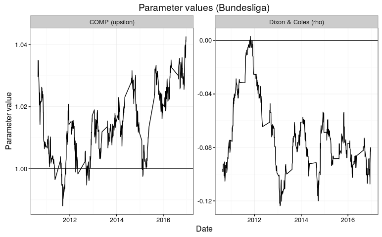
I have also found a relatively simple formula for BTTS probability for the Dixon-Coles model. Recall that the Dixon-Coles model applies an adjustment to low scoring outcomes (less than two goals scored by either team), shifting probabilities to (or from) 0-0 and 1-1 to 1-0 and 0-1 outcomes. The amount of probability that is shifted depends on the parameter called rho. For the BTTS probability, it is the adjustment to the probability of the 1-1 outcome that is of interest. The trick is basically to subtract the probability of the 1-1 outcome for the underlying independent model without the Dixon-Coles adjustment, and then add back the Dixon-Coles adjusted 1-1 probability. The Dixon-Coles adjustment for the 1-1 outcome is simply 1 – rho, which does not depend on the expected goals of the two sides.

Here is some R code that shows how to apply the adjustment:


# Dixon-Coles adjustment parameter.
rho <- 0.13

# 1-1 probability for the independent Poisson model.
p11 <- dpois(1, lambda = expg1) * dpois(1, lambda = expg2) 

# Add DC adjusted 1-1 probability, subtract unadjusted 1-1 probability.
dc_correction <- (p11 * (1-rho)) - p11

# Apply the corrections
prob_btts_dc  <- prob_btts_2 + dc_correction

If you run this, you will see that the BTTS probability decreases to 55.4% when rho = 0.13.

I have added two functions for computing BTTS probabilities in the new version 0.6 of the goalmodel package, so be sure to check that out. The predict_btts() function works just like the other predict_* functions in the package, where you give the function a fitted goalmodel, together with the fixtures you want to predict, and it gives you the BTTS probability. The other function is pbtts(), which works independently of a fitted goalmodel. Instead you just give it the expected goals, and other paramters like the Dixon-Coles rho parameter, directly.

Expected goals from over/under odds

I got a comment the other day asking about whether it is possible to get the expected number of goals scored from over/under odds, similar to how you can do this for odds for win, draw or lose outcomes. The over/under odds refer to the odds for the total score (the sum of the score for two opponents) being over or under a certain value, usually 2.5 in soccer.

It is possible, and rather easy even, to get the expected total score from the over/under odds, at least if you assume that the number of goals scored by the two teams follows a Poisson distribution. This is the same assumption that makes the method for extracting the expected goals from HDW odds possible. The Poisson distribution is really convenient and reasonable realistic probability model for different scorelines. It is controlled by a single parameter, called lambda, that is also the expected value (and the expected goals in this case). One convenient property of the Poisson is that the sum of two Poisson distributed variables with parameters lambda1 and lambda2 is also Poisson distributed, with the lambda being the sum of the two lambdas, i.e. lambdasum = lambda1 + lambda2.

So how can you find the expected total number of goals based on the over/under odds? First you need to convert the odds for the under outcome to a proper probability. How you do this depends on the format your odds come in, but in R you can use the odds.converter package to convert them to decimal format, and then use my own package called implied to convert them to proper probabilities.

After you have the probabilities for the under probability, you can use the Poisson formula to find the value of the parameter lambda that gives the probability for the under outcome that matched the probability from the odds. In R you can use the built-in ppois function to compute the probabilities for there being scored less than 2.5 goals when the expected total goals is 3.1 like this:

under <- 2.5
ppois(floor(under), lambda=3.1)

This will give us that the probability is 40.1% of two or less goals being scored in total, when the expected total is 3.1. Now you can try to manually adjust the lambda parameter until the output matches your probability from the odds. Another way is to automate this search using the built-in uniroot function. The uniroot function takes as input another function, and searches for the input value that gives the result 0. We therefore have to write a function that takes as input the expected goals, the probability implied by the odds, and the over/under limit, and returns the difference between the probability from the Poisson model and the odds probability. Here is one such function:

obj <- function(expg, under_prob, under){
  (ppois(floor(under), lambda=expg) - under_prob)
}

Next we feed this to the uniroot function, and gives a realistic search interval for the expected goals, between 0.01 and 10 in this case, and the rest of the parameters. For this example I used 62% chance of there being scored less than 2.5 goals.

uniroot(f = obj,
        interval = c(0.01, 10),
        under_prob = 0.62,
        under = 2.5)

From this I get that the expected total goals is 2.21.

You might wonder if it is possible to get the separate expected goals for the two teams from over/under odds using this method. This is unfortunately not possible. The only thing you can hope for is to get a range of possible values for the two expected goals that sums to the total expected goals. In our example with the expected total goals being 2.21, the range of possible values for the two expected goals can be plotted as a line like this:

If course, you can judge some pairs of expected goals being more likely than others, but there is no information about this in over/under odds alone. It might be possible, I am not 100% sure, that other non-Poisson models, which would involve more assumptions, could exploit the over/under odds to get expected goals for both teams.

The probabilities implied by bookmaker odds: Introducing the ‘implied’ package

My package for converting bookmaker odds into probabilities is now on available from CRAN. The package contains several different conversion algorithms, which are all accessible via the implied_probabilities() function. I have written an introduction on how you can use the package here, together with a description of all the methods and with references to papers. But I also want to give some background to some of the methods here on the blog as well.

In statistics, an odd is usually taken to mean the inverse of a probability, that is 1/p, but in the betting world different odds formats exists. As usual, Wikipedia has a nice overview of the different formats. In the implied package, only inverse probability odds are allowed as inputs, which in betting are called decimal odds.

Now you might think that converting decimal odds to probabilities should be easy, you can just use the definition above and take the inverse of the odds to recover the probability. But it is not that simple, since in practice using this simple formula will give you improper probabilities. They will not sum to 1, as they should, but be slightly larger. This gives the bookmakers an edge and the probabilities (which aren’t real probabilities) can not be considered fair, and so different methods for correcting this exists.

Some methods uses different types of regression modelling combined with historical data to estimate the biases in the different outcomes. This is for example the case in the paper On determining probability forecasts from betting odds by Erik Štrumbelj. Anyway, the implied package does not include these kinds of methods. The reason I wanted to mention this paper is that this was where I first read about Shin’s method for the first time.

All the methods in the package are what I call one-shot methods. The conversion of a set of odds for a game only relies on the odds them self, and not on any other data. This is deliberate choice, since I didn’t want to make a modelling package, since that would be much more complicated.

Many of the methods in the package comes are described in the Wisdom of the Crowd document by Joseph Buchdahl, and a review paper by Clarke et al (Adjusting Bookmaker’s Odds to Allow for Overround).

Many of the methods in the package can be described as ad hoc methods. They basically use a simple mathematical formula that relates the true underlying probabilities to the improper probabilities given by the bookmakers odds. Then this formula is used to find the true probabilities so that they are proper (sum to 1) while also recovering the improper bookmaker probabilities.

A few other methods in the package are more theory based, like Shin’s method, and I find these methods really interesting. Shin’s method imagine that there are two types of bettors. The first type is the typical bettor, and the sum of bets by this type follows the “wisdom of the crowd” pattern which should reflect the true ncertainty of the outcome given the publicly available information. Then there is a second type of bettor, which has inside information and always bets on the winning outcome. However, the bookmaker don’t know what type of bettor the individual bettors are, and only observes the mixture of the two types. Here is the interesting part: By assuming the bookmakers know that there are two types of bettors, and that the bookmakers seek to maximize their profits, Shin was able to derive some complicated formulas that relate the true underlying “wisdom of the crowds” probabilities and the bookmakers odds. These formulas can be used in the same way as the ad hoc methods to find the underlying probabilities.

A natural question question is what method gives the most realistic probabilities? There is no definite answer to this, and different methods will be best in different markets and settings. You need to figure this out for yourself.

I am currently working on some new methods inspired by Shin’s framework which I hope to write about later. Shin’s work was mostly done in the context of horse racing, where there is realistic that some bettors have inside information. I hope to develop a method that is more relevant for football.

Expected goals from bookmaker odds

I recently read an interesting paper called The Betting Odds Rating System: Using soccer forecasts to forecast soccer by Wunderlich and Memmert. In their paper they develop av variant of the good old Elo rating system. Instead of using the actual outcomes of each match to calculate the ratings, they use the probabilities of the outcomes, which they get from bookmaker odds.

I was wondering if a similar approach could be used together with the goalmodel package I released a couple of months ago. The models available in the package are models I have written about extensively on this blog, and they all work as follows: You use the number of goals scored to get some ratings of the goal scoring and goal conceding rates of each team. You then use these ratings to forecast the expected number of goals in the upcoming games. These expected goals can then be used to calculate the probabilities of the outcome (Home win, draw, away win). A crucial step in these calculations is the assumption that the number of goals scored follow the Poisson distribution (or some related distribution, like the Negative Binomial).

But can we turn this process the other way around, and use bookmaker odds (or odds from other sources) to get expected goals and maybe also attack and defense ratings like we do in the goalmodel package? I think this is possible. I have written a function in R that takes outcome probabilities and searches for a pair of expected goals that matches the probabilities. You can find it on github (Edit: The function is now included in the goalmodel package.). This function relies on using the Poisson distribution.

Next, I have expanded the functionality of the goalmodel package so that you can use expected goals for model fitting instead of just observed goals. This is possible by setting the model argument to “model = ‘gaussian'” or to “model = ‘ls'”. These two options are currently experimental, and are a bit unstable, so if you use them, make sure to check if the resulting parameter estimates make sense.

I used my implied package to convert bookmaker odds from the 2015-16 English Premier League into probabilities (using the power method), found the expected goals, and then fitted a goalmodel using the least squares method. Here are the resulting parameters, from both using the expected goals and observed goals:

I wanted to use this season for comaprison as this was the season Leicester won unexpectedly, and in the Odds-Elo paper (figure 6) it seemed like the ratings based on the odds were more stable than the ones based on the actual results, which increased drastically during the season. In the attack and defense ratings from the goalmodels we see that Leicester have average ratings (which is what ratings close to 0 are) in the model based on odds, and much higher ratings based on the actual results. So the goalmodel and Elo ratings seem to agree, basically.

I also recently discovered another paper titled Combining historical data and bookmakers’odds in modelling football scores, that tries something similar as I have done here. They seem to do the same extraction of the expected goals from the bookmaker odds as I do, but they don’t provide the details. Instead of using the expected goals to fit a model, they fit a model based on actual scores (similar to what the goalmodel package do), and then they take a weighted average of the model based expected goals and the expected goals from the bookmaker odds.

Introducing the goalmodel R package

I have written a lot about different models for forecasting football results, and provided a lot of R code along the way. Especially popular are my posts about the Dixon-Coles model, where people still post comments, four years since I first wrote them. Because of the interest in them, and the interest in some of the other models I have written about, I decided to tidy up my code and functions a bit, and make an R package out of it. The result is the goalmodel R package. The package let you fit the ordinary Poisson model, which was one of the first models I wrote about, the Dixon-Coles model, The Negative-Binomial model, and you can also use the adjustment I wrote about in my previous update.

The package contains a function to fit the different models, and you can even combine different aspects of the different models into the same model. You can for instance use the Dixon-Coles adjustment together with a negative binomial model. There is also a range of different methods for making prediction of different kinds, such as expected goals and over/under.

The package can be downloaded from github. It is still just the initial version, so there are probably some bugs and stuff to be sorted out, but go and try it out and let me know what you think!

A small adjustment to the Poisson model that improves predictions.

There are a lot extensions to the basic Poisson model for predicting football results, where perhaps the most popular is the Dixon-Coles model which I and other have written a lot about. One paper that seem to have received little attention is the 2001 paper Prediction and Retrospective Analysis of Soccer Matches in a League by Håvard Rue and Øyvind Salvesen (preprint available here). The model they describe in the paper extend the Dixon-Coles and Poisson model in several ways. The most interesting extension in how they allow the attack and defense parameters vary over time, by estimating a separate set of parameters for each match. This might at first seem like a task that should be impossible, but they manage to pull it of by using some Bayesian magic that let the estimated parameters borrow information across time. I have tried to implement something similar like this in Stan, but I haven’t gotten it to work quite right, so that will have to wait for another time. There’s many other interesting extensions in the paper as well, and here I am going to focus on one of of them which is an adjustment for teams to over and underestimate opponents when they differ in strengths.

The adjustment is added to the formulas for calculating the log-expected goals. So if team A plays team B at home, the log-expected goals \(\lambda_A\) and \(\lambda_B\)

\( \lambda_A = \alpha + \beta + attack_{A} – defense_{B} – \gamma \Delta_{AB} \)

\( \lambda_B = \alpha + attack_{B} – defense_{A} + \gamma \Delta_{AB} \)

In these formulas are \(\alpha\) the intercept, \(\beta\) the home team advantage and \(\Delta_{AB}\) is a factor that determines the amount a team under- or overestimation the strength of the opponent. This factor is given as

\(\Delta_{AB} = (attack_{A} + defense_{A} – attack_{B} – defense_{B}) / 2\)

The parameter \(\gamma\) determines how large this effect is. A positive \(\gamma\) implies that a strong team will underestimate a weak opponent, and thereby score fewer goals than we would otherwise expect, and vice versa for the opponent.

In the paper they do not estimate the \(\gamma\) parameter directly together with the other parameters, but instead set it to a constant, with a value they determine by backtesting to maximize predictive ability.

When I implemented this model in R and estimated it using Maximum Likelihood I noticed that adding the adjustment did not improve the model fit. I suspect that this might be because the model is nearly unidentifiable. I even tried to add a Normal prior on \(\gamma\) and get a Maximum a Posteriori (MAP) estimate, but then the MAP estimate were completely determined by the expected value of the prior. Because of these problems I decided to use a different strategy: I estimated the model without the adjustment, but add the adjustment when making predictions.

I am not going to post any R code on how to do this, but if you have estimated a Poisson or Dixon-Coles model, it should not be that difficult to add the adjustment when you calculate the predictions. If you are going to use some of the code I have posted on this blog before, you should notice the important detail that in the formulation above I have followed the paper and changed the signs of the defense parameters.

In the paper Rue and Salvesen write that \(\gamma = 0.1\) seemed to be an overall good value when they analyze English Premier League data. To see if my approach of adding the adjustment only when doing predictions is reasonable I did a leave-one-out cross validation on some seasons of English Premier League and German Bundesliga. I fitted the model to all the games in a season, except one, and then add the adjustment when predicting the result of the left out match. I did this for several values of \(\gamma\) to see which values works best.

Here is a plot of the Ranked Probability Score (RPS), which is a measure of prediction accuracy, against different values of \(\gamma\) for the 2011-12 Premier League season:

As you see I even tried some negative values of \(\gamma\), just in case. At least in this season the result agrees with the estimate \(\gamma = 0.1\) that Rue and Salvesen reported. In some of the later seasons that I checked the optimal \(\gamma\) varies somewhat. In some seasons it is almost 0, but then again in some others it is around 0.1. So at least for Premier league, using \(\gamma = 0.1\) seems reasonable.

Things are a bit different in Bundesliga. Here is the same kind of plot for the 2011-12 season:

As you see the optimal value here is around 0.25. In the other seasons I checked the optimal value were somewhere between 0.15 and 0.3. So the effect of over- and underestimating the opponent seem to be greater in the Bundesliga than in Premier League.

A simple re-implementation of the Dixon-Coles model

A couple of years ago I implemented the Dixon-Coles model for predicting football results here on this blog. That series of of blog posts is my most popular since I keep getting comments on it, some four years later.

One of the most common requests is advice on how to expand the model to include additional predictors. Unfortunately with the implementation I posted this was not so straightforward. It relied on some design matrices with dummy-coded variables, which is a standard way of doing things in regression modeling. The DC model isn’t a standard regression modeling problem, so using matrices complicated things. I posted some updates and variant across several posts, which in the end made the code a bit hard to follow and to modify.

Anyway, I’ve had a simpler implementation lying around for a while, and since there’s been far between updates on this blog lately I thought I’d post it.

First load some data from the engsoccerdata package. I’m going to use the 2011-12 season of the English Premier League, so the results can be compared with what I got from the first implementation.

library(dplyr)
library(engsoccerdata)

england %>% 
  filter(Season == 2011,
         tier==1) %>% 
  mutate(home = as.character(home),
         visitor = as.character(visitor))-> england_2011

Next we should create a list of initial parameter values. This will be used as a starting point for estimating the parameters. The list contains vectors of four groups of parameters, the attack and defense parameters of all teams, the home field advantage and the Dixon-Coles adjustment (rho). The attack and defense vector are named so that it is easy to look up the relevant parameter later on.

Notice also that a sum-to-zero constraint has to be added to the defense parameters, so in reality we are estimating one defense parameter less than the number of teams. Check this post for some more explanation of this.

# Make a vector of all team names. 
all_teams <- sort(unique(c(england_2011$home, england_2011$visitor)), decreasing = FALSE)
n_teams <- length(all_teams)

# list of parameters with initial values.
parameter_list <- list(attack = rep(0.2, n_teams),
                      defense = rep(-0.01, n_teams-1),
                      home = 0.1,
                      rho= 0.00)

names(parameter_list$attack) <- all_teams
names(parameter_list$defense) <- all_teams[-1] # the first parameter is computed from the rest.

Next we need a function that calculates the negative log-likelihood function, to be used with R’s built in optimizer.

One trick I use here is to relist the parameters. The optimizer want all parameter values as a single vector. When you have a lot of parameters that group together and is used in different parts of the model, this can quickly create some complicated indexing and stuff. By supplying the original parameter list, plus having named vectors, these problems essentially disappear.

Also notice how the expected goals are now simply computed by looking up the relevant parameters in the parameter list and adding them together. No need for matrix multiplications.

The Dixon-Coles adjustment function tau is the same as in the original implementation.

dc_negloglik <- function(params, goals_home, goals_visitor,
                     team_home, team_visitor, param_skeleton){
  
  # relist, to make things easier.
  plist <- relist(params, param_skeleton)
  
  # There is a sum-to-zero constraint on defense parameters.
  # The defense parameter for the first team is computed from the rest.
  plist$defense <- c(sum(plist$defense)*-1, plist$defense)
  names(plist$defense)[1] <- names(plist$attack[1]) # add name to first element.

  # Home team expected goals
  lambda_home <- exp(plist$attack[team_home] + plist$defense[team_visitor] + plist$home)
  
  # Away team expected goals
  lambda_visitor <- exp(plist$attack[team_visitor] + plist$defense[team_home])
  
  # Dixon-Coles adjustment
  dc_adj <- tau(goals_home, goals_visitor, lambda_home, lambda_visitor, rho = plist$rho)
  
  # Trick to avoid warnings.
  if (any(dc_adj <= 0)){
    return(Inf)
  }
  
  # The log-likelihood
  log_lik_home <- dpois(goals_home, lambda = lambda_home, log=TRUE)
  log_lik_visitor <- dpois(goals_visitor, lambda = lambda_visitor, log=TRUE)
  
  log_lik <- sum((log_lik_home + log_lik_visitor + log(dc_adj)))
  
  return(log_lik*-1)
  
}

To actually estimate the parameters we feed the function, data and initial values to optim, and check the results.


optim_res <- optim(par = unlist(parameter_list), fn=dc_negloglik,
                   goals_home = england_2011$hgoal,
                   goals_visitor = england_2011$vgoal,
                   team_home = england_2011$home, team_visitor = england_2011$visitor,
                   param_skeleton=parameter_list, method = 'BFGS')

# relist, and calculate the remaining parameter. 
parameter_est <- relist(optim_res$par, parameter_list)
parameter_est$defense <- c( sum(parameter_est$defense) * -1, parameter_est$defense)
names(parameter_est$defense)[1] <- names(parameter_est$attack[1]) 

I get the same home field advantage (0.27) and rho (-0.13) as in the original implementation. The other parameters differ, however. This is because of the sum-to-zero constraints are coded in a different way. This should not matter and both ways should give the same predictions.

I have not yet said anything about how to expand the model to include other predictors, but hopefully this implementation should make it easier. You can just add some new arguments to the dc_negloglik function that takes the variables in question as input, and add new parameter vectors to the parameter list as needed. Then the calculations of the expected goals should be modified to include the new parameters and predictors.

Which model is the best?

I had a discussion on Twitter a couple of weeks ago about which model is the best for predicting football results. I have suspected that the Dixon & Coles model (DC), which is a modification of the Poisson model, tend to overfit. Hence it should not generalize well and give poorer predictions. I have written about one other alternative to the Poisson model, namely the Conway-Maxwell Poisson model (COMP). This is a model for count data that can be both over-, equi- and underdispersed. It is basically a Poisson model but without the assumption that the variance equals the mean. I have previously done some simple analyses comparing the Poisson, DC and COMP models, and concluded then that the COMP model was superior. The analysis was however a bit to simple, so I have now done a more proper evaluation of the models.

A proper way to evaluatie the models is to do a backtest. For each day there is a game played, the three models are fitted to the available historical data (but not data from the future, that would be cheating) and then used to predict the match outcomes for that day. I did this for two leagues, the English Premier League and German Bundesliga. The models were fitted to data from both the top league and the second tier divisions, since this improves the models, but only the results of the top division was predicted and used in the evaluation. I used a separate home field advantage for the two divisions and the rho parameter in the DC model and the dispersion parameter in the COMP model was estimated using the top division only.

To measure the model’s predictive ability I used the Ranked Probability Score (RPS). This is the proper measure to evaluate predictions for the match outcome in the form of probabilities for home win, draw and away win. The range of the RPS goes from 0 (best possible predictions) to 1 (worst possible prediction). Since the three models actually model the number of goals, I also looked at the probability they gave for the actual score.

For all three models I used the Dixon & Coles method to weight the historical data that is used in training the models. This requires tuning. For both the English and German leagues I backtested the models on different values of the weighting parameter \(\xi\) on the seasons from 2005-06 to 2009-10, with historical data available from 1995. I then used the optimal \(\xi\) for backtesting the seasons 2010-11 up to December 2016. This last validation period covers 1980 Bundesliga matches and 2426 Premier League matches.

Here are the RPS for the three models plottet against \(\xi\). Lower RPS is better and lower \(\xi\) weights more recent data higher.

xi epl

xi bundesliga

The graphs show a couple of things. First, all three models have best predictive ability at the same value of \(\xi\), and that they compare similarly also for non-optimal values of \(\xi\). This makes things a bit easier since we don’t have to worry that a different value of \(\xi\) will alter our evaluations about which model is the best.

Second, there is quite some difference between the models for the German and English data. In the English data the COMP model is clearly best, while the DC is the worst. In the German league, the DC is clearly better, and the COMP and Poisson models are pretty much equally good.

So I used the optimal values of \(\xi\) (0.0021 and 0.0015 for Premier League and Bundesliga, respectively) to validate the models in the data from 2010 and onwards.

Here is a table of the mean RPS for the three models:

rps table

We see that for the both English Premier League and German Bundesliga the DC model offers best predictions. The COMP model comes second in Premier League, but has worst performance in the Bundesliga. It is interesting that the DC model performed worst in the tuning period for the Premier League, now was the best one. For the Bundesliga the models compared similarly as in the tuning period.

I also looked at how often the DC and COMP models had lower RPS than the Poisson model. The results are in this table:

compare with poisson

The COMP model outperformed the Poisson model in more than 60% of the matches in both leagues, while the DC model did so only about 40% of the time.

When looking at the goal scoring probabilities. Here is a table of the sum of the minus log probabilities for the actual scoreline. Here a lower number also indicates better predictions.

score log probabilities

Inn both the Premier League and Bundesliga the Poisson model was best, followed by COMP, with the DC model last.

We can also take a look at the parameter values for the extra parameters the DC and COMP models has. Remember that the DC models is becomes the Poisson model when rho = 0, while the COMP model is the same as the Poisson model when upsilon = 1, and is underdispersed when upsilon is greater than 1.

params ger

params epl

The parameter estimates fluctuates a bit. It is intersting to see that the rho parameter in the DC model tend to be below 1, which gives the opposite direction of what Dixon and Coles found in their 1997 paper. In the Premier League, the parmater makes a big jump to above 0 at the end of the 2013-14 season. The parameter appears to be a bit more consistent in the Bundesliga, but also there we see a short period where the parameter is around 0.

The dispseriosn parameter upsilon also isn’t all that consistent. It is generally closer to 1 in the Bundesliga than in the Premier League. I think this is consistent with why this model was better in the Premier League than in the Bundesliga.

All inn all I think it is hard to conclude which of the three models is the best. The COMP and DC models both adjusts the Poisson model in their own specific ways, and this may explain why the different ways of measuring their predictive abilities are so inconsistent. The DC model seem to be better in the German Bundesliga than in the English Premier League. I don’t think any of the two models are generally better than the ordinary Poisson model, but it could be worthwhile to look more into when the two models are better, and perhaps they could be combined?

The comparison graph part 2

In the last post I wrote about how a graph could be used to explore an important aspect of a data set of football matches, namely whom has played against whom. In this post I will present a more interesting graph. Here is how a graph of 4500 international matches, including friendlies, world cups, and continental cups, from 2010 to 2015:

intgr1

There are 214 teams in this data set, each represented by a circle, and if two teams has played against each other, there is a line drawn between the two circles. It becomes clear when we see this graph that the graph is complicated, with a lot of lines between the circles, and it is hard to make a drawing that shows the structure really well.

There are a few things we can see clearly, though. The first is that the graph is highly connected. All teams are at least indirectly comparable with all other teams. There are no unconnected subgraphs. One measure of how connected the graph is, is the average number of edges the nodes have. In this graph this number is 23.2, which means that each team has on average played against 23 other teams.

On interesting thing we also notice is the “arm” on the right side of the plot, with a handful of teams that is more or less separated from the rest of the teams. These are teams from the Pacific nations, such as Fiji, Samoa and Cook Islands and so on.

In a data set like this we can find some interesting types of indirect comparisons. One example I found in the above graph was Norway and Japan, who has not played against each other in the five year period the data spans, but they have both played against two other teams that link them together: Zambia and Greece.

intgr_norjap

I haven’t found a decent measure of the overall connectedness between two nodes, that incorporates all indirect links of all degrees, but that could be an interesting thing to look at.

Another thing we can do with a graph like this is a cluster analysis. A cluster analysis gives us a broader look at the connectedness in the graph by finding groups of nodes that are more connected to each other that to those in the other groups. In other words we are trying to find groups of countries that play against each other a lot.

A simple clustering of the graph gives the following clusters, with some of the country names shown. The clustering algorithm identified 5 clusters that rather perfectly corresponds to the continents. This is perhaps not so surprising since the continental competitions (including the World Cup qualifications) make up a large portion of the data.

intgr_cluster

Tuning the Elo ratings: Initial ratings and inter-league matches

In the last post I discussed how to tune the Elo ratings to make the ratings have the best predictive power by finding the optimal update factor (the K-factor) and adjustment for home field advantage. One thing I only mentioned, but did not go into detail about, was that the teams initial ratings will influence this tuning. In this post I will show how we can find good initial ratings that also will mitigate some other problems associated with Elo ratings.

As far as I can tell, setting the initial ratings does not seem to be much discussed. The Elo system updates the ratings by looking at the difference between the actual results and the results predicted by the rating difference between the two opposing teams. To get this to work in the earliest games in the data, you need to supply some initial ratings.

It is possible to set the initial ratings by hand, using your knowledge about the strengths of the different players and teams. This strategy is however difficult to use in practice, since you may not have that knowledge, which in turn would give incorrect ratings. This task would also become more difficult the more teams and players are in your data. An automatic way to get the initial ratings is of course preferable.

The only automatic way to set the initial ratings I have seen is to set all ratings to be equal. This is what they do at FiveThirtyEight. This simple strategy is obviously not optimal. It is a bit far fetched to assume that all teams are equally good at the beginning of your data, even if you could argue that you don’t really know any better. If you have a lot of data going back a long time, then only the earliest period of your ratings will be unrealistic. After a while the ratings will become more realistic and better reflect the true strengths of the teams.

The unrealistic ratings for the earliest data may also cause a problem if you use this to find the optimal K-factor. In Elo ratings the K-factor is a parameter that determines how much new games will influence the ratings. A larger K-factor makes the ratings change a lot after a new game, while a low K-factor will make the ratings change only a little after each new game. If you are trying to make a rating system with good prediction ability and use the earliest games with the unrealistic ratings to tune the K-factor, then it will probably be overestimated. This is because a large K-factor will make the ratings change a lot at the beginning, making the ratings better quicker. A large K-factor will be good in the earliest part of your data, but after a while it may be unrealistically big.

One more challenge with Elo ratings is if you include multiple leagues or competitions in your rating system. Since the Elo ratings are based on the exchange of points, groups of teams that play each other often, such as the teams in the same league, will have ratings that are reasonable calibrated only between each other. This is not the case when you have teams from different leagues play each other. The rating difference between two teams from two leagues will not be as well-calibrated as those within a league.

A nice visualization of this is to plot which teams in your data have played each other. In the plot below each team is represented by a circle, and each line between the circles indicates that the two teams have against played each other. The data is from Premier League and the Championship from the year 2010; two half-seasons for each division. I haven’t added team names to the graph, but the orange circles are the teams that played in the Premier League in both seasons, while the blue circles are teams that played in the Championship or got promoted or relegated.

comparison graph2 crop

We clearly see that the two division cluster together with a lot of comparisons available between the teams. Six teams, those that got promoted and relegated between the two divisions, are clearly shown to fall in between the two large clusters. All comparisons to be made between teams in the two divisions has to rely on the information that is available via these six teams. Including all these teams in a Elo rating, starting with all ratings equal, will surely be completely wrong and will take some time to be realistic. All point exchange between the divisions will have to happen via the promoted and relegated teams.

I have previously investigated this in the context of regression models, where I demonstrated how including data from the Championship improves the prediction of Premier League matches. Se this and this.

So how can we find the initial ratings that will give realistic ratings that also calibrate the ratings between two or more leagues? By using a small amount of data, say one year worth of data, less that you would use to tune the K-factor and home field advantage, you can use an optimization algorithm to find the ratings that best fits the observed outcomes. In doing this you have to use the formula that converts the ratings to expected outcomes, but you do not use the update formula, so this approach can be seen as a static version of the Elo ratings.

Doing the direct optimization is however not completely straightforward. Elo ratings is a zero-sum system. No points are added or removed from the system, only exchanged. This constraint is similar to the sum-to-zero constraint that is sometimes used in regression modeling and Analysis-of-Variance. To overcome this, we can simply set the rating of one of the teams to the negative sum of the ratings of all the other teams.

A further refinement is to include home field advantage into the optimization. In cases where the teams have unequal number of home games, or some games where no teams play at home, this will create more accurate ratings. If not the ratings for those teams with an excess of home games will become unrealistically large.

Doing this procedure, using data from the Premier League and the Championship from 2010 which I used to make the graph above, I get the following ratings (with the average rating being 1500):

elo inits

The procedure also estimated the home field advantage to be 84.3 points.

The data I used for the initial ratings is the first year of the data I used to tune the K-factor in the previous post. How does using these initial ratings influence the this tuning, compared with using the same initial rating for all teams? As expected, the optimal K-factor is smaller. The plot below shows that K=14 is the optimal K, compared with K=18.5 that I found last time. It is also interesting to see that the ratings with initialization are more accurate for the whole range of K’s I tested, than those without.

kwithinit