The Elo rating system is quite simple, and therefore easy implement. In football, FIFA uses is in its womens rankings and the well respected website fivethirtyeight.com also uses Elo ratings to make predictions for NBA and NFL games. Another cool Elo rating site is clubelo.com.
Three year ago I posted some R code for calculating Elo ratings. Its simplicity also makes it easy to modify and extend to include more realistic aspects of the games and competitions that you want to make ratings for, for example home field advantage. I suggest reading the detailed description of the clubelo ratings to get a feel of how the system can be modified to get improved ratings. I have also discussed some ways to extend the Elo ratings here on this blog as well.
If you implement your own variant of the Elo ratings it is necessary to tune the underlying parameters to make the ratings as accurate as possible. For example, a too small K-factor will give ratings that update too slow. The ratings will not adapt well to more recent developments. Vice versa, a too large K-factor will put too much weight on the most recent results. The same goes for the extra points added to the home team rating to account for the home field advantage. If this is poorly tuned, you will get poor predictions.
In order to tune the rating system, we need a way to measure how accurate the ratings are. Luckily the formulation of the Elo system itself can be used for this. The Elo system updates the ratings by looking at the difference between the actual results and the results predicted by the rating difference between the two opposing teams. This difference can be used to tune the parameters of the system. The smaller this difference is, the more accurate are the predictions, so we want to tune the parameters so that this difference is as small as possible.
To formulate this more formally, we use the following criterion to assess the model accuracy:
where \(exp_{hi}\) and \(exp_{ai}\) are the expected results of match i for the home team and the away team, respectively. These expectations are a number between 0 and 1, and is calculated based on the ratings of the two teams. \(obs_{hi}\) and \(obs_{ai}\) are the actual result of match i, encoded as 0 for loss, 0.5 for draw and 1 for a win. This criterion is called the squared error, but we will use the mean squared error.
With this criterion in hand, we can try to find the best K-factor. Using data from the English premier league as an example I applied the ratings on the match results from the January 1st 2010 to the end of the 2014-15 season, a total of 2048 matches. I tried it with different values of the K-factor between 7 and 25, in 0.1 increments. Then plotting the average squared error against the K-factor we see that 18.5 is the best K-factor.

The K-factor I have found here is, however, probably a bit too large. In this experiment I initialized the ratings for all teams to 1500. This includes the teams that was promoted from the Championship. A more realistic rating system would initialize these teams with a lower rating, perhaps be given the ratings from the relegated teams.
We can of course us this strategy to also find the best adjustment for the home field advantage. The simple way to add the home field advantage is to add some additional points to the ratings for the home team. Here I have used the same number of points in all matches across all season, but different strategies are possible. To find the optimal home field advantage I applied the Elo ratings with K=18.5, using different home field advantages.
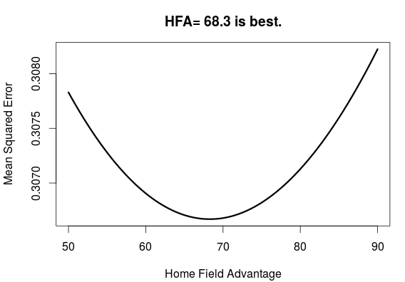
From this plot we see that an additional 68.3 points is the optimal amount to add to the rating for the home team.
One might wonder if finding the best K-factor and home field advantage independent of each other is the best way to do it. When I tried to find the best K-factor with the home field advantage set to 68, I found that the best K was 19.5. This is a bit higher than when the home field advantage was 0. I tried to find the optimal pair of K and home field advantage by looking over a grid of possible values. Plotting the accuracy of the ratings against both K and the home field advantage in a contour we get the following:

The best K and home field advantage pair can be read from the plot, both of which is a bit higher than the first values I found.
Doing the grid search can take a bit of time, especially if you don’t narrow down the search space by doing some initial tests beforehand. I haven’t really tried it out, but alternating between finding the best K-factor and home field advantage and using the optimal value from the previous round is probably going to be a reasonable strategy here.