In the last post I wrote about how a graph could be used to explore an important aspect of a data set of football matches, namely whom has played against whom. In this post I will present a more interesting graph. Here is how a graph of 4500 international matches, including friendlies, world cups, and continental cups, from 2010 to 2015:

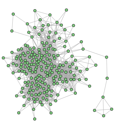
There are 214 teams in this data set, each represented by a circle, and if two teams has played against each other, there is a line drawn between the two circles. It becomes clear when we see this graph that the graph is complicated, with a lot of lines between the circles, and it is hard to make a drawing that shows the structure really well.

There are a few things we can see clearly, though. The first is that the graph is highly connected. All teams are at least indirectly comparable with all other teams. There are no unconnected subgraphs. One measure of how connected the graph is, is the average number of edges the nodes have. In this graph this number is 23.2, which means that each team has on average played against 23 other teams.

On interesting thing we also notice is the “arm” on the right side of the plot, with a handful of teams that is more or less separated from the rest of the teams. These are teams from the Pacific nations, such as Fiji, Samoa and Cook Islands and so on.

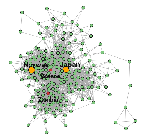
In a data set like this we can find some interesting types of indirect comparisons. One example I found in the above graph was Norway and Japan, who has not played against each other in the five year period the data spans, but they have both played against two other teams that link them together: Zambia and Greece.

I haven’t found a decent measure of the overall connectedness between two nodes, that incorporates all indirect links of all degrees, but that could be an interesting thing to look at.

Another thing we can do with a graph like this is a cluster analysis. A cluster analysis gives us a broader look at the connectedness in the graph by finding groups of nodes that are more connected to each other that to those in the other groups. In other words we are trying to find groups of countries that play against each other a lot.

A simple clustering of the graph gives the following clusters, with some of the country names shown. The clustering algorithm identified 5 clusters that rather perfectly corresponds to the continents. This is perhaps not so surprising since the continental competitions (including the World Cup qualifications) make up a large portion of the data.