
In part 1 I wrote about the basics of the Poisson regression model for predicting football results, and briefly mentioned how our data should look like. In this part I will look at how we can fit the model and calculate probabilities for the different match outcomes. I will also discuss some problems with the model, and hint at a few improvements.
Fitting the model with R
When we have the data in an appropriate format we can fit the model. R has a built in function glm() that can fit Poisson regression models. The code for loading the data, fitting the model and getting the summary is simple:
#load data
yrdta <- read.csv(“yourdata.csv”)

#fit model and get a summary
model <- glm(Goals ~ Home + Team + Opponent, family=poisson(link=log), data=yrdta)
summary(model)
The summary function for fitting the model with data from Premier League 2011-2012 season gives us this (I have removed portions of it for space reasons):
(Edit September 2014: There was some errors in the estimates in the original version of this post. This was because I made some mistakes when I formated the data as described in part one. Thanks to Derek in the comments for pointing this out. )
Coefficients:
                    Estimate Std. Error z value Pr(>|z|)
(Intercept)          0.45900    0.19029   2.412 0.015859 *
Home                 0.26801    0.06181   4.336 1.45e-05 ***
TeamAston Villa     -0.69103    0.20159  -3.428 0.000608 ***
TeamBlackburn       -0.40518    0.18568  -2.182 0.029094 *
TeamBolton          -0.44891    0.18810  -2.387 0.017003 *
TeamChelsea         -0.13312    0.17027  -0.782 0.434338
TeamEverton         -0.40202    0.18331  -2.193 0.028294 *
TeamFulham          -0.43216    0.18560  -2.328 0.019886 *
-----
OpponentSunderland  -0.09215    0.20558  -0.448 0.653968
OpponentSwansea      0.01026    0.20033   0.051 0.959135
OpponentTottenham   -0.18682    0.21199  -0.881 0.378161
OpponentWest Brom    0.03071    0.19939   0.154 0.877607
OpponentWigan        0.20406    0.19145   1.066 0.286476
OpponentWolves       0.48246    0.18088   2.667 0.007646 **
---
Signif. codes:  0 ‘***’ 0.001 ‘**’ 0.01 ‘*’ 0.05 ‘.’ 0.1 ‘ ’ 1
The Estimate column is the most interesting one. We see that the overall mean is e0.49 = 1.63 and that the home advantage is e0.26 = 1.30 (remember that we actually estimate the logarithm of the expectation, therefore we need to exponentiate the coefficients to get interpretable numbers). If we want to predict the results of a match between Aston Villa at home against Sunderland we could plug the estimates into our formula, or use the predict() function in R. We need to do this twice, one time to predict the number of goals Aston Villa is expected to score, and one time for Sunderland.
#aston villa
predict(model, data.frame(Home=1, Team="Aston Villa", Opponent="Sunderland"), type="response")
# 0.9453705

#for sunderland. note that Home=0.
predict(model, data.frame(Home=0, Team="Sunderland", Opponent="Aston Villa"), type="response")
# 0.999
We see that Aston Villa is expected to score on average 0.945 goals, while Sunderland is expected to score on average 0.999 goals. We can plot the probabilities for the different number of goals against each other:
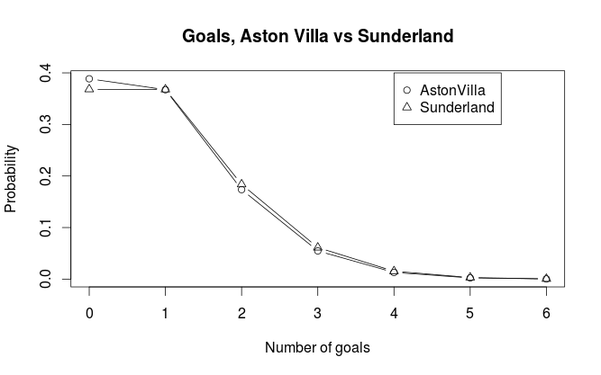
We can see that Aston Villa has just a bit higher probability for scoring not goals than Sunderland. Sunderland has also just a tiny bit higher probablity for most other number of goals. Both teams have about the same probability of scoring exactly one goal. In general the pattern we see in the plot is consistent with what we would expect considering the expected number of goals.
Match result probabilities
Now that we have our expected number of goals for the two opponents in a match, we can calculate the probabilities for either home win (H), draw (D) and away win (A). But before we continue, there is an assumption in our model that needs to be discussed, namely the assumption that the goals scored by the two teams are independent. This may not be obvious since surely we have included information about who plays against who when we predict the number of goals for each team. But remember that each match is included twice in our data set, and the way the regression method works, each observation are assumed to be independent from the others. We’ll see later that this can cause some problems.
The most obvious way calculate the probabilities of the three outcomes is perhaps to look at goal differences. If we can calculate the probabilities for goal differences (home goals minus away goals) of exactly 0, less than 0, and greater than 0, we get the probabilities we are looking for. I will explain two ways of doing this, both yielding the same result (in theory at least): By using the Skellam distribution and by simulation.
Skellam distribution
The Skellam distribution is the probability distribution of the difference of two independent Poisson distributed variables, in other words, the probability distribution for the goal difference. R does not support it natively, but the VGAM package does. For our example the distribution looks like this:
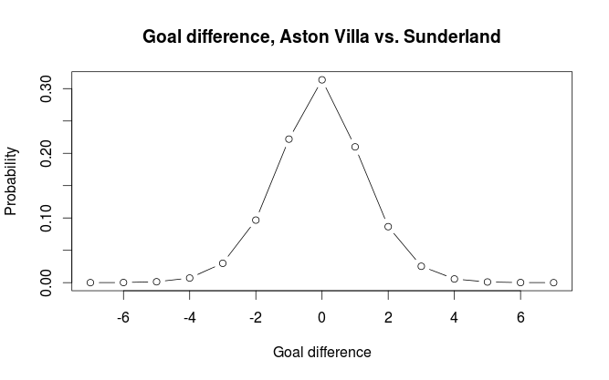
If we do the calculations we get the probabilities for home win, draw, away win to be 0.329, 0.314, 0.357 respectively.
#Away
sum(dskellam(-100:-1, predictHome, predictAway)) #0.3574468
#Home
sum(dskellam(1:100, predictHome, predictAway)) #0.3289164
#Draw
sum(dskellam(0, predictHome, predictAway)) #0.3136368
Simulation
The second method we can use is simulation. We simulate a number of matches (10000 in our case) by having the computer draw random numbers from the two Poisson distributions and look at the differences. We get the probabilities for the different outcomes by calculating the proportion of different goal differences. The independence assumption makes this easy since we can simulate the number of goals for each team independently of each other.
 set.seed(915706074)
nsim <- 10000
homeGoalsSim <- rpois(nsim, predictHome)
awayGoalsSim <- rpois(nsim, predictAway)
goalDiffSim <- homeGoalsSim - awayGoalsSim
#Home
sum(goalDiffSim > 0) / nsim #0.3275
#Draw
sum(goalDiffSim == 0) / nsim # 0.3197
#Away
sum(goalDiffSim < 0) / nsim #0.3528
The results differ a tiny bit from what we got from using the Skellam distribution. It is still accurate enough to not cause any big practical problems.
How good is the model at predicting match outcomes?
The Poisson regression model is not considered to be among the best models for predicting football results. It is especially poor at predicting draws. Even when the two teams are expected to score the same number of goals it rarely manages to assign the highest probability for a draw. In one attempt I used Premier League data from the last half of one season and the first half of the next season to predict the second half of that season (without refitting the model after each match day). It assigned highest probability to the right outcome in 50% of the matches, but never once predicted a draw.
Lets see at some other problems with the model and suggest some improvements.
One major problem I see with the model is that the predictor variables are categorical. This is a constraint that makes inefficient use of the available data since we get rather few data points per parameter (i.e per team). The model does for example not understand teams are more like each other than others and instead view each team in isolation. There has been some attempts at using Bayesian methods to incorporate information on which teams are better and which are poorer. Se for example this blog. If the teams instead could be reduced to numbers (by using some sort of rating system) we would get fewer parameters to estimate. We could then also incorporate an interaction term, something that is almost impossible with the categorical predictor variables we have. The interaction term in this case would be the effect of a team under or over estimating its opponent.
(As an aside, we could in fact interpret the coefficients in our model as a form of rating of a teams offensive and defensive strength)
Another way the model can be improved is to incorporate a time aspect. The most obvious way to do this is perhaps to weights to the matches such that more recent matches are more important than matches far back in time.
A further improvement would be to look at the level of different players, and not at a team as a whole. For example will a team with many injured players in a match most likely perform poorer than what you would expect. One could use weights to down weight the contribution of matches where this is a problem. A much more powerful idea would be to combine data on match lineup with a rating system for players. This could be used to infer a rating for the whole team in a specific match. In addition to correct for injured players it would also account for new players on a team and players leaving a team. The biggest problem with this approach is lack of available data in a format that is easy to handle.
I don’t think any of the improvements I have discussed here will solve the problem of predicting draws since it originates in the independent Poisson assumption, although I think they could improve predictions in general. To counter the problem of predicting draws I think a very different model would have to be used. I would also like to mention that the improvements I have suggested here are rather general, and could be incorporated in many other prediction models.
hi there,
Was wondering if you could provide the code you used to produce the charts for the probability of Aston Villa and Sunderland goals
Here is how I did it. You need the VGAM package installed to make the goal difference plot.
#expected number of goals for both teams predictHome <- predict(model, data.frame(Home=1, Team="Aston Villa", Opponent="Sunderland"), type="response") predictAway <- predict(model, data.frame(Home=0, Team="Sunderland", Opponent="Aston Villa"), type="response") #plot the poisson distributions plotrange <- 0:6 hp <- dpois(plotrange, predictHome) ap <- dpois(plotrange, predictAway) plot(plotrange, hp, type="b", ylim=range(hp, ap), main="Goals, Aston Villa vs Sunderland", xlab="Number of goals", ylab="Probability") points(plotrange, ap, type="b", pch=24) legend(x=4, y=0.4, legend=c("AstonVilla", "Sunderland"), pch=c(21, 24)) #Goal difference, skellam distribution goalDiffRange <- -7:7 plot(goalDiffRange, dskellam(goalDiffRange, predictHome, predictAway), type="b", main="Goal difference, Aston Villa vs. Sunderland", ylab="Probability", xlab="Goal difference")Hi,
Why Arsenal (both Team and Opposition) is not shown?
It has to do with how R encodes categorical variables. By default R uses the first level as a baseline which all other levels are compared with. I forgot about it while I wrote the post, but I think it would be better to use contr.sum as the coding method.
Also, see this: http://stackoverflow.com/questions/2352617/how-and-why-do-you-use-contrasts-in-r
Hi,
How to calculate overall mean and the home advantage factor from the output of glm() that contains, Error pr and Z value etc
Estimate Std. Error z value Pr(>|z|)
(Intercept) 0.490383 0.187268 2.619 0.00883 **
Home 0.268009 0.061807 4.336 1.45e-05 ** what it actually means?
You should exponentiate the numbers in the estimate column, as I explained in the post, right under the output.
Hi,
Cool analysis! I use the data from England Premier League 2011-2012 to run the R code, but the summary is different, is this possible? Here is my part of output:
Coefficients:
Estimate Std. Error z value Pr(>|z|)
(Intercept) 0.45900 0.19029 2.412 0.015859 *
Home 0.26801 0.06181 4.336 1.45e-05 ***
TeamAston Villa -0.69103 0.20159 -3.428 0.000608 ***
TeamBlackburn -0.40518 0.18568 -2.182 0.029094 *
TeamBolton -0.44891 0.18810 -2.387 0.017003 *
TeamChelsea -0.13312 0.17027 -0.782 0.434338
TeamEverton -0.40202 0.18331 -2.193 0.028294 *
TeamFulham -0.43216 0.18560 -2.328 0.019886 *
TeamLiverpool -0.46401 0.18675 -2.485 0.012969 *
…..
That is weird. At least the home field advantage is approximately the same. There’s a number of steps where you could have made a mistake (or I could have made a mistake). Are you sure you put your data in the format described in part 1, so that each match is seen as two observations? Did you use the half time score instead of the full time score? Did we use different data sources, and one had some mistakes? Did you use the
glmfunction with Poisson log-link instead of thelmfunction?Hi,
Great article as commented above 🙂
While trying to user predict function with same data I am experiencing an error. Also tried with Spanish Liga data and happening the same, not sure if it’s related to changes to the function since the article was writting. Do you know why? any alternative? Thanks in advance and keep posting!
> predict(model_Premier, data.frame(Home=1, Team=”Aston Villa”, Opponent=”Sunderland “), type=”response”)
Error in model.frame.default(Terms, newdata, na.action = na.action, xlev = object$xlevels) :
factor Opponent has new level Sunderland
According to the error message you are trying to predict the results of a game with a team that you don’t have any previous data on (Sunderland). Try to predict the results using other teams for which you have data.
predict(model_Premier, data.frame(Home=1, Team=”Aston Villa”, Opponent=”Sunderland “), type=”response”)
See the Opponent, there are a space behind Sunderland, it might be the reason.
Good article. If anyone’s interested, http://scoreline.tips has a nice graphical tool that shows the Poisson distribution of scorelines for any match, with means based on current data. It also lets you change the input means and watch the table update in real-time.
That’s a cool visualization. I like how you can adjust the probabilities based on your own subjective considerations (aka “expert knowledge”). Do you use a model similar to the one I described here? With ” optimal combination of current and previous season matches”, do you mean you do a weighted regression? If so, how did you calculate the weights?
Hi,
thanks for this great article. I was trying to do something simiilar but as Tom mentions before Arsenal (both home and away) is not shown.
Is there a way to let Arsenal be shown and the other not be compared to Arsenal?
Will the esitmation of Team and Opponent not change if we compare to other team than Arsenal? And therefore the odds of goals scored by each team will change?
You can specify which team you want to use as baseline (which team the other teams will be compared against, “control group” in scientific terms) by doing something like this, which sets the fifth team (in alphabetical order) as the baseline:
Since there is no natural team that can be regarded as the baseline, I prefer to use the sum-to-zero contranst. Unfortunately the summary function in R does not provide the names of the teams in the output when you use this. You can however get the parameters for all attack parameters if you remove the intercept parameter and use the sum-to-zero contrast:
How exactly you do it does not matter if you use the predict function, the contrasts serve two purposes. One, because of some mathematical details I will not go into, you have to specify the contrasts for the estimation algorithm to find a unique set of parameters. Second, the different types of contrasts serves as tools to help the interpretation of the parameters. But, as I said, if you are mostly interested in making predictions, you shouldn’t worry too much.
Hi, I’ve done the above advise about using contr.sum, however there still isn’t a row for “opponentArsenal” giving the defensive strength of them. How do we obtain that?
If you add Opponent=”contr.sum” to the list in the contrasts argument, you will get the one parameter for each opponent as well. Unfortunately, R does not give the team names (I don’t know why), but Arsenal will typically be the Opponent1 (they are sorted alphabetically). To verify you can add x=TRUE to the glm function, and check model$x afterwards to verify that the matches where Arsenal is the opponent is indicated so in the opponent columns.
I didn’t this row model <- glm(Goals ~ Home + Team + Opponent – 1, family=poisson(link=log), data=yrdta, contrasts=list(Team="contr.sum"))
summary(model).
Why opponent – 1 ?
Adding -1 to the formula removes the intercept.
I didn’t understand how can one build the dataset.
Can you post a sample spreadsheet on the blog, please?
If you download data from http://www.football-data.co.uk/ in csv format you can either do the manipulations I explained in part 1 with spreadsheet software (excel or open office) or use the small snippet of code I posted here
Hi there,
I ran into your document on the internet, I couldn’t understand much of it but what caught my interest is your believability that it is possible to predict football match results….
I will like to know if you have little time for me to share what I have with you…
There is another way to predict football draws but there is no way to document it because academia isn’t my strong forte….
I would like to know if you are conversant with R or Weka or Rapid Miner?
My method of prediction is crude and I would like to know if you and I can brainstorm on how to engage machine learning techniques to increase chances of predicting the right football match result….
If this discussion interests you, please get back to me.
Iamshuga@gmail.com
I got the result as below base on re-format file.
Coefficients:
Estimate Std. Error z value Pr(>|z|)
(Intercept) 0.490383 0.187268 2.619 0.00883 **
Home 0.268009 0.061807 4.336 1.45e-05 ***
TeamAston Villa -0.241067 0.200472 -1.203 0.22917
TeamBlackburn 0.052390 0.186929 0.280 0.77927
TeamBolton 0.096123 0.184704 0.520 0.60277
TeamChelsea 0.128518 0.182632 0.704 0.48162
It is not the same as your posted. but it seems match your documents 0.49 and 0.26 in the next paragraph.
which is the exact one?
Sorry, I got my mistake, I forget to exchange the TEAM and Opponent.
BTW, 0.49 and 0.26 should change to the correct value.
Thanks.
Great article! Was wondering if a bivariate Poisson distribution would solve the problems you mentioned, and if you can do another one of your tutorials on that? 🙂
Yes, it might! I have a series of posts on the Dixon-Coles model, and also the COM-model, which I think will interest you.
Do you have or know some code for Bivariate Poisson?
Hi! Thanks for a great post!
I tried to do the same to data from La Liga in season 15-16 but I seem to be getting negative prediction of goal amounts. Any thoughts on how that’s possible? The piece of code is below and I can’t seem to find what I’m doing differently.
> model predict(model, data.frame(home=1, team=”Ath Madrid”, opponent=”Barcelona”, type=”response”))
1
0.1129038
> predict(model, data.frame(home=0, team=”Barcelona”, opponent=”Ath Madrid”, type=”response”))
1
-0.1897685
In addition it seems that I’m not getting any kind of response by using type in the predict command. I always get the same answer whether it’s “response” or “term” or nothing at all. Also my model summary looks the same no matter if I use poisson or quasipoisson as “family”.
If you have any idea why this is so, help is appreciated.
And noticed I had misplaced parenthesis… How blind can one be regardless the effort.
Thank you! The quasipoisson is, if I have understood it correctly, just a trick to correct the standard errors of the parameter estimates if there is under- or over-dispersion. The coefficients should be the same, but in the bottom of the model summary you should see a line which gives the dispersion parameter if you use the quasi-poisson.
Thanks for the reply! I’m under the same impression.
Btw. I would like to ask about a part in your text: “Even when the two teams are expected to score the same number of goals it rarely manages to assign the highest probability for a draw.”
Isn’t it only rational, that the model never assigns the highest probability for a draw, since it would not be the most probable case even when teams were completely equally matched? At least this is how I understand it and it’s quite intuitive too, since the game can end in so many more ways in favor of one or another than it can as a draw.
I guess that is one way of putting it, but it will of course depend on the probabilities of all those other results. With the poisson model it turns out that way, but with the Dixon-Coles model for example, you get higher probability of a draw (although i am not sure in what, if any, situations it will give the highest probability for draw).
So I am not sure if it is completely rational, or intuitive, that a model should automatically give low probability for a draw. An ideal model would reflect the true probabilities of the results (to the degree it makes sense to talk about true probabilities), even if that would mean giving high probability for a draw. Of course models are not ideal, and for what I know a draw might rarely be the most probable result in football anyway.
Hi, when you said you’d plug the estimates into the formula, what did you mean by it? And if I were to do this without R, how will this work? What will the mean be for the poisson distribution?
Thank you
You take the parameter estimates from the model, and plug them into the formula in part 1. The formula is rather simple. If you want to predict the number of goals that Aston Villa will score against Sunderland you add together the attack (or Team) parameter for Villa and the defense (or Opponent) parameter for Sunderland, plus the intercept. If Villa play at home you add the home field advantage parameter as well. Then you exponentiate it to get the expected number of goals for Villa. You can of course do this (fit the model, do the predictions) with some other software than R. Poisson regression should be standard in most statistics software.
I meant is it possible to do poisson regression without any coding/statistics software? Is it possible to do this with regression analysis in excel and through poisson distribution?
Excel do have some functions for the Poisson distribution, but I am not sure if there are any regression modeling routines. It should be possible to implement a Possison regression model in Excel using a combination of the Poisson distribution and the built-in optimization routines. Some quick googling also gives some commercial add-ons that can do it.
Hi, I enjoyed the article ref poisson distribution model to predict match results. Would you be able to share a basic model with us?
Thank you.
Ryan
Yeah, it is described here: http://opisthokonta.net/?p=276
Hi,
I am doing a research project on predicting PL football results. I am wondering how you calculated the team coefficients? Forgive me if you have mentioned this already.
Thank you,
Natalie
They are calculated with the glm function.
Hello,
Thank you for this nice blog. It’s really useful and it helped me a lot to create a similar model in Matlab. I’ve got three short questions:
1) I’ve some issues with adding a low score correction to this model. Would it in your opinion also be ok to make a “correction matrix”? E.g, I know the real goal distribution and I know the average predicted score matrix (averaged over a whole season). The ratio between the two would be my correction matrix?…
2) I’ve read on pena.lt/y an article about draw predictions and why they are low in general. His statement is basically that a model should rarely predict a chance for a draw >31%. This is a bit in contradiction with your statements about draws (even when the same team is playing against each other). What’s your opinion about that article?
3) How to add the time weight to this model? We do not use the DClog function…
Best regards,
Leon
PS: I want to learn more about statistics and data analysis in my spare time. Can you recommend on what would be a good starting point (e.g a free online course) 🙂
Thank you!
I think I discussed some alternative correction matrices in the comments under some other post one time. I don’t remember exactly which one. On idea that I had, which was inspired by a link someone posted, was to interpolate between the overage observed score probabilities (po) and the predicted score probabilties (pp):
v * po + (1-v)*pp
Where the parameter v selects between the model predictions and the simple observed probabilities. I haven’t tested this out, so I cant say if it gives better predictions.
About the draws, I don’t quite see the contradiction? With a Poisson model the larges probabilities for a draw would be when two equally strong teams who both will score almost no goals.
I don’t know of any specific online courses i could recommend, but I know there are a lot of resources out there. Depending on on what your prior knowledge of programming and maths are, I could recommend the book Elements of Statistical Learning. It is more about machine learning techniques and not data analysis in general though.
Hello,
Your blog is excellent. please how do i use the Poisson regression model with the goalmodel using update datasets. it will be interesting to see how the goalmodel improves the performance of the regression model.
thank you.
I am not sure what you mean by update datasets.
thanks for your prompt response. i did the following trying to predict next upcoming epl games using England_current function according to engsoccerdata/R/england_current.R
england_2018 <- function(Season=2018) …………….
Then did this
gm_res <- goalmodel(goals2 = england_2018$hgoal, goals1 = england_2018$vgoal,
+ team2 = england_2018$home, team1=england_2018$visitor)
result out
Error in length(goals1) == length(goals2) :
object of type 'closure' is not subsettable
kindly assist. thank you
It seems you are defining a function called england_2018, and then pass this to the goalmodel function as if it was a data frame.
How can I put time-weighted in this model?
Hey, great article, I tried utilizing the exact same data as you did and copied the code to see how it was running, but I keep getting this error where the opponent coefficients don’t generate and 10 not defined because of singularities. Any help would be greatly appreciated thanks.
Did you use the example data from part 1? That is only 5 games, not enough to fit a model. As a rule of thumb you should have at least one season of data, or at least 2 or 3 games per team.
Hi, I have a question, I tried to train my model using data from two leagues, so that I can predict matches for next year and have estimators for teams that have been promoted. The problem is that I am getting NA in my estimator for one team. Can you figure out what am I doing wrong?
sorry for the long code block
#################################################
prepare_data = function(dataframe) {
dataframe = dataframe[c(“HomeTeam”, “AwayTeam”, “FTHG”, “FTAG”)]
dataframe.temp = dataframe[, c(2,1,4)]
names(dataframe.temp) = c(“HomeTeam”, “AwayTeam”, “Goals”)
dataframe = dataframe[c(“HomeTeam”, “AwayTeam”, “FTHG”)]
names(dataframe) = c(“HomeTeam”, “AwayTeam”, “Goals”)
dataframe = rbind(dataframe, dataframe.temp)
dataframe$Home<- rep(c(1,0), each = nrow(dataframe) / 2)
dataframe
}
# try to train model using two leagues
mydata3a <- read.csv("https://www.football-data.co.uk/mmz4281/1718/E0.csv", header = TRUE, stringsAsFactors = TRUE)
mydata3b <- read.csv("https://www.football-data.co.uk/mmz4281/1718/E1.csv", header = TRUE, stringsAsFactors = TRUE)
mydata3a = prepare_data(mydata3a)
mydata3b = prepare_data(mydata3b)
mydata3 = rbind(mydata3a, mydata3b)
model <- glm(Goals ~ Home + HomeTeam + AwayTeam -1, family=poisson,
data=mydata3, contrasts=list(AwayTeam="contr.sum"))
The problem is probably that you don’t have any data between the leagues. You have basically two clusters of teams that are not comparable. Two possible solutions is 1) to add more data, possibly from the season previous seasons, or the FA cup, 2) fit two separate models.
I have discussed this in the context of Elo rating: http://opisthokonta.net/?p=1412
Hi, nice blog. I am enjoying reading your articles on predicting football games.
I was wondering if you could provide the code on how you ” In one attempt I used Premier League data from the last half of one season and the first half of the next season to predict the second half of that season (without refitting the model after each match day). ” I am unsure on how to predict outcomes for more than one game at a time.
Many thanks
You can either use a loop, or give all the games you want to predict to the predict function in the form of a data frame.
Hi, I wanted to ask how would I use this predictor in new data to read in a league season and predict the following season with the new teams. Also do you have any code for a Skellam regression model. thanks
With this model, which uses only team names, it is impossible to make predictions for new teams not in the data used to fit the model. You can try to include more data from the division where the new teams are promoted from, for example. I don’t have any code for a Skellam regression model.
I tested it with scipy python package using its PoissonRegressor (https://scikit-learn.org/stable/modules/generated/sklearn.linear_model.PoissonRegressor.html#sklearn-linear-model-poissonregressor). The D^2 score, percentage of deviance explained, was 0.028741994178717367 and the mean deviance (caculated by https://scikit-learn.org/stable/modules/generated/sklearn.metrics.mean_poisson_deviance.html) was 1.140599386446271. I don’t know how to interpret it, how bad is that?
Using the goalmodel package, the explained variance tend to be around 0.15. Getting 0.03 seems bad, but I am not completly sure they are the same quantity.
Hi,
wonderful job.
Do you think it would be possible to include more variables to the model for example goals and xG or goals and shots. If it is, how would it be done in R?
Just provide the data in an additional covariate matrix?
Many thanks!
Yes that would be possible. I see some only use average goals for and against, xg, etc for the last 5 or 10 games as predictors, for example. Using the glm function would be straight forward, provided you have organized the data correctly.
Splendid! If you have time could you provide an example of how to incorporate, for example, your mentioned additional predictors in glm() function in R. Is it possible to just add those variables to your readymade goalmodel() function?
You need to stack the data so that each match is represented with two rows, as is shown in part 1. You can use additional covariates in the goalmodel function. The github page for the package explains how to do it. You need to store the data in two matrices (one for home and one for away) and give them via the x1 and x2 arguments.
I am sorry, I’m quite late to the party. I haven’t been able to get my head around how to fit for one half of the season and then predict for the second half. I would be grateful if you could provide a code for that. It would be very helpful.
You can divide the data.frame in two, the first part which you use to fit the model, and the next you use with the predict function.
I am sorry, but would you be able to provide a line of code showing how to split the data.frame into 2. I tried understanding the goal model package, but I’m new to R so pretty stuck. It would be quite helpful
With my last post I was little hasty. The Poisson model based on xGoals was not yet ready, but now. Unfortunately, there is an error message. The cause is probably the decimal data type of xGoals. Is it possible to fit the model so that xGoals are also accepted?
> gm_res_dc warnings()
Warnmeldungen:
1: In dpois(y, mu, log = TRUE) : non-integer x = 1.200000
2: In dpois(y, mu, log = TRUE) : non-integer x = 1.200000
3: In dpois(y, mu, log = TRUE) : non-integer x = 1.500000
Yes, to use decimal numbers, set model = ‘gaussian’ when you use the goalmodel function. More information here:
https://github.com/opisthokonta/goalmodel#the-gaussian-model
Thanks, I hadn’t seen that.
I have another question. Is it possible to load several leagues at once (e.g. English Premier League and German Bundesliga)? This is necessary if I want to predict a match between Bayern Munich and Arsenal.
Regards
Yes you can do that, but it might give you an error. If you just give data from to separate leagues it wont work, unless you have some data to “bridge” the two leagues, such as data from the champions league.
I also got the error when trying to process two leagues at once. It could have been that there is a workaround.
I use your goalmodel (default poisson with hfa and dc). I am missing a matrix plot (goals from 0 to 5) that shows the most likely scoreline. Here you can see what I mean (step 6). Is there a way to create such a table?
https://www.sbo.net/strategy/football-prediction-model-poisson-distribution/
Yes, you first need to make a prediction using the predict_goals() function. To inspect it more closely, i prefer to plot it using ggplot2. If you use the function with return_df=TRUE, you get a data.frame with the probabilities that you can use with ggplot2. Here is a quick draft of how the code could look like. I havent run this exact code myself, so it might not work, but is should give you an idea on how to do it.
my_pred_df <- predict_goals(... ... ... , return_df=TRUE) ggplot(my_pred_df, aes(x = goals1, y = goals2, color = probability, label = probability)) + geom_tile() + geom_text() You may need to do something extra steps to round the displayed probabilities to only 2 decimals or something, and maybe also not display goals > 5 or something.
Hello! Thanks for the info especially where you said improving Poisson model using line ups and player data. I’m looking forward to implement one,I arleady managed to scrape player xG data in a match from understats.com but I’m confused how to start but I have an idea of first getting team expected goal as usual and normalising average player(starting xi) scoring rates to get each player expected goals in a match to eventually use Poisson to predict each player scoring probabilities I will later use in Monte Carlo simulations for the market probabilities. Am I missing something here?
Hi,
this is a great implementation.
When i tried doing this, I tried it across a couple of seasons. My biggest issue is how to handle teams newly relegated and newly promoted during prediction since there will be no co-efficients for those.
any suggestions?
Yes that is often a bit difficult. One way would be to just make up some data. Take a look at how promoted teams do against the best and worst teams from the previous season, and then just include some typical fake data points based on the history of promoted/relegated teams. Maybe also include some data from the previous season in the division below. Also take a look at the discussion here: https://opisthokonta.net/?p=1108
Additionally, I was thinking if we can inject a Variable in our data (still unsure how) to denote that the 2 rows are dependent, would that make a better model than the current one?
Also, how can one get in touch with you?
I dont it is easy to simply add a variable as predictor to somehow account for the fact that each match shows up twice in the setup bescribed in the post. There are some models that can have model bivariate correlations, such as the Dixon-Coles model. You can fit the DC model with the goalmodel R package that i made that you can install from here:
https://github.com/opisthokonta/goalmodel
Other models, which are not in goalmodel, could also be possible, such as a bivariate poisson model. Not sure about any package that fits those kinds of models.