Underdispersed Poisson alternatives seem to be better at predicting football results

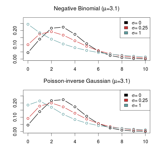
In the previous post I discussed some Poisson-like probability distributions that offer more flexibility than the Poisson distribution. They typically have an extra parameter that controls the variance, or dispersion. The reason I looked into these distributions was of course to see if they could be useful for modeling and predicting football results. I hoped in particular that the distributions that can be underdispersed would be most useful. If the underdispersed distributions describe the data well then the model should predict the outcome of a match better than the ordinary Poisson model.

The model I use is basically the same as the independent Poisson regression model, except that the part with the Poisson distribution is replaced by one of the alternative distributions. Let the \(Y_{ij}\) be the number of goals scored in game i by team j


\( Y_{ij} \sim f(\mu_{ij}, \sigma) \)
\( log(\mu_{ij}) = \gamma + \alpha_j + \beta_k \)

where \(\alpha_j\) is the attack parameter for team j, and \(\beta_k\) is the defense parameter for opposing team k, and \(\gamma\) is the home field advantage parameter that is applied only if team j plays at home. \(f(\mu_{ij}, \sigma)\) is one of the probability distributions discussed in the last post, parameterized by the location parameter mu and dispersion parameter sigma.

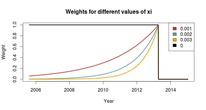
To these models I fitted data from English Premier League from the 2010-11 season to the 2014-15 season. I also used Bundesliga data from the same seasons. The models were fitted separately for each season and compared to each other with AIC. I consider this only a preliminary analysis and I have therefore not done a full scale testing of the accuracy of predictions where I refit the model before each match day and use Dixon-Coles weighting.

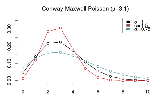
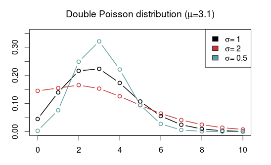
The five probability distributions I used in the above model was the Poisson (PO), negative binomial (NBI), double Poisson (DPO), Conway-Maxwell Poisson (COM) and the Delaporte (DEL) which I did not mention in the last post. All of these, except the Conway-Maxwell Poisson, were easy to fit using the gamlss R package. I also tried two other gamlss-supported models, the Poisson inverse Gaussian and Waring distributions, but the fitting algorithm did not work properly. To fit the Conway-Maxwell Poisson model I used the CompGLM package. For good measure I also fitted the data to the Dixon-Coles bivariate Poisson model (DC). This model is a bit different from the rest of the models, but since I have written about it before and never really tested it I thought this was a nice opportunity to do just that.

The AIC calculated from each model fitted to the data is listed in the following table. A lower AIC indicates that the model is better. I have indicated the best model for each data set in red.

Pois_alt_aic

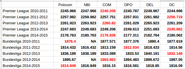
The first thing to notice is that the two models that only account for overdispersion, the Negative Binomial and Delaporte, are never better than the ordinary Poisson model. The other and more interesting thing to note, is that the Conway-Maxwell and Double Poisson models are almost always better than the ordinary Poisson model. The Dixon-Coles model is also the best model for three of the data sets.

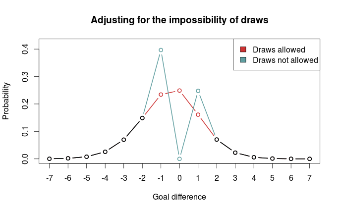
It is of course necessary to take a look at the estimates of the parameters that extends the three models from the Poisson model, the \(\sigma\) parameter for the Conway-Maxwell and double Poisson and the \(\rho\) for the Dixon-Coles model. Remember that for the Conway-Maxwell a \(\sigma\) greater than 1 indicates underdispersion, while for the Double Poisson model a \(\sigma\) less than 1 is indicates underdispersion. For the Dixon-Coles model a \(\rho\) less than 0 indicates an excess of 0-0 and 1-1 scores and fewer 0-1 and 1-0 scores, while it is the opposite for \(\rho\) greater than 0.

pois_alt_params

It is interesting to see that the estimated dispersion parameters indicate underdispersion for all the data sets. It is also interesting to see that the data sets where the parameter estimates are most indicative of equidispersion is where the Poisson model is best according to AIC (Premier League 2013-14 and Bundesliga 2010-11 and 2014-15).

The parameter estimates for the Dixon-Coles model do not give a very consistent picture. The sign seem to change a lot from season to season for the Premier League data, and for the data sets where the Dixon-Coles model was found to be best, the signs were in the opposite direction of what where the motivation described in the original 1997 paper. Although it does not look so bad for the Bundesliga data, this makes me suspect that the Dixon-Coles model is prone to overfitting. Compared to the Conway-Maxwell and double Poisson models that can capture more general patterns in all of the data, the Dixon-Coles model extends the Poisson model to just parts of the data, the low scoring outcomes.

It would be interesting to do fuller tests of the prediction accuracy of these three models compared to the ordinary Poisson model.

Some alternatives to the Poisson distribution

One important characteristic of the Poisson distribution is that both its expectation and the variance equals parameter \(\lambda\). A consequence of this is that when we use the Poisson distribution, for example in a Poisson regression, we have to assume that the variance equals the expected value.

The equality assumption may of course not hold in practice and there are two ways in which this assumption can be wrong. Either the variance is less than the expectation or it is greater than the expectation. This is called under- and overdispersion, respectively. When the equality assumption holds, it is called equidispersion.

There are two main consequences if the assumption does not hold: The first is that standard errors of the parameter estimates, which are based on the Poisson, are wrong. This could lead to wrong conclusions when doing inference. The other consequence happens when you use the Poisson to make predictions, for example how many goals a football team will score. The probabilities assigned to each number of goals to be scored will be inaccurate.

(Under- and overdispersion should not be confused with heteroscedasticity in ordinary linear regression. Poisson regression models are naturally heteroscedastic because of the variance-expectation equality. Dispersion refers to what relationship there is between the variance and the expected value, in other words what form the heteroscedasticity takes.)

When it comes to modeling and predicting football results using the Poisson, a good thing would be if the data were actually underdispersed. That would mean that the probabilities for the predicted number of goals scored would be higher around the expectation, and it would be possible to make more precise predictions. The increase in precision would be greatest for the best teams. Even if the data were really overdispersed, we would still get probabilities that more accurately reflect the observed number of goals, although the predictions would be less precise.

This is the reason why I have looked into alternatives to the Poisson model that are suitable to model count data and that are capable of being over- and underdispersed. Except for the negative binomial model there seems to have been little focus on more flexible Poisson-like models in the literature, although there are a handful of papers from the last 15 years with some applied examples.

I should already mention the gamlss package, which is an extremely useful package that can fit a large number of regression type models in R. I like to think of it as the glm function on steroids. It can be used to create regression models for a large number of distributions (50+) and using different forms of dependent variables (for example random effects and splines) and doing regression on distribution parameters other than the usual expectation parameters.

The models that I have considered usually have two parameters. The two parameters are often not easy to interpret, but the distributions can be re-parameterized (which is done in the gamlss package) so that the parameters describe the location (denoted \(\mu\), often the same as the expectation) and shape (denoted \(\sigma\), often a dispersion parameter that modifies the association between the expectation and variance). Another typical property is that they equal the Poisson for certain values of the shape parameter.

As I have already mentioned, the kind of model that is most often put forward as an alternative to the Poisson is the Negative binomial distribution (NBI). The advantages of the negative binomial are that is well studied and good software packages exists for using it. The shape parameter \(\sigma > 0\) determines the overdispersion (relative to the Poisson) so that the closer it is to 0, the more it resembles the Poisson. This is a disadvantage as it can not be used to model underdispersion (or equidispersion, although in practice it can come arbitrarily close to it). Another similar, but less studied, model is the Poisson-inverse Gaussian (PIG). It too has a parameter \(\sigma > 0\) that determines the overdispersion.

NBI_PIG

A large class of distributions, called Weighted Poisson distributions, is capable of being both over- and underdispersed. (The terms Weighted in the name comes from a technique used to derive the distribution formulas, not that the data is weighted) A paper describing this class can be found here. The general form of the probability distribution is

\(P(x;\theta,\alpha)=\frac{e^{\mu x+\theta t(x)}}{x!C(\theta,\alpha)}\)

where \(t(x)\) is one of a large number of possible functions, and \(C(\theta,\alpha)\) is a normalizing constant which makes sure all probabilities in the distribution sum to 1. Note that I have denoted the two parameters using \(\theta\) and \(\alpha\) and not \(\mu\) and \(\sigma\) to indicate that these are not necessarily location and shape parameters. I think this and interesting class of distributions that I want to look more into, but since they are not generally implemented in any R package that I know of I will not consider them further now.

Another model that is capable of being over- and underdispersed is the Conway–Maxwell–Poisson distribution (COM), which incidentally is a special case of the class of Weighted Poisson distributions mentioned above (see this paper). The Poisson distribution is a special case of the COM when \(\sigma = 1\), and is underdispersed when \(\sigma > 1\) and overdispersed when \(\sigma\) is between 0 and 1. One drawback with the COM model is that the expected value depends on both parameters \(\mu\) and \(\sigma\), although it is dominated by \(\mu\). This makes the interpretation a bit difficult, but it may not be a problem when making predictions.

Unfortunately, the COM model is not supported by the gamlss package, but there are some other R packages that implements it. I have tried a few of them and the only one that I got to work is CompGLM, which for some reason does not use the location (\(\mu\)) and shape (\(\sigma\)) parameterization.

COM

The Double Poisson (DP) is another interesting distribution which also equals the Poisson distribution when \(\sigma = 1\), but is overdispersed when \(\sigma > 1\) and underdispersed when \(\sigma\) is between 0 and 1. The expectation does not depend on the shape parameter \(\sigma\), and it is approximately equal to the location parameter \(\mu\). Another interesting thing about the Double Poisson is that it is belongs to a larger group of distributions called double exponential families which also lets you derive a binomial-like distribution with an extra dispersion parameter which can be useful in a logistic regression setting (see this paper, or this preprint).

DP

In a follow up post I will try to use these distributions in regression models similar to the independent Poisson model.

A hectic schedule has some effect on the outcome of a football match

It may be that a football team who has had a hectic period with a lot of games will, because of lack of training and restitution, perform poorer. The Wikipedia page for the FA Cup mentions Manchester United’s absence from the cup as a reason for why they won the Premier League by 18 points in the 1999-2000 season. If this is indeed the case, then this is something we could try to exploit in a prediction model.

I basically used the same data and model as I have used before. I used data from the English Championship and the Premier League, and predicted the Premier League games from January 2007 until January 2015 using the independent Poisson model with the Dixon & Coles weighting method (more details on the setup here and here). In addition I constructed a new variable, the number of matches each team has played the last x number of days, were we can use and try different values of x. As a pretentious shorthand I will call this the Match Schedule Intensity Index (MSII). Matches from the FA Cup, Europa Cup and Champions League were also included in the calculations.

As usual I used the ranked probability score (RPS) to assess the prediction accuracy.

I tried four different number of days back in time: 21, 25, 28 and 31 days. I also varied the time weighing parameter \(\xi\) a bit to see how these things varied together.

Plotting the RPS, number of days back in time and the different values of \(\xi\) against each other gives the following:

xiRPS

We see that looking back 28 days in time gives the lowest RPS and this the most accurate predictions of the four alternatives. 25 days is almost as good as 28 days, while 21 and 31 days performs poorer than not having the MSII in the model at all. I am not sure how important the drop in RPS is, as the changes are around the 4th and 5th decimal place. It is probably not that much, but on the other hand, this is an average over 3000 matches, and the number of days back in time seems to be a more important parameter than the small changes in \(\xi\) that I tried.

It is also interesting to see what effect the MSII has on the number of goals scored. I plotted the estimated multiplicative effect for each additional match for all the fitted models from 2007 to 2015 using the best model with 28 days and \(\xi=0.0020\).

effectTime

I expected the effect of additional matches to be negative, meaning the more games the team has recently played, the fewer goals will they be expected to score. This seems to be at least halfway true, except for a few dips over on the positive side around 2010 and 2013-2014, and a rather large positive effect from the start in 2007 until 2008. This was a bit surprising, and I don’t know why. It would be interesting to redo the analysis with data going further back in time to see how far back the positive effect goes.

Is the effect large? Not really. The most extreme values of the multiplicative effects for the MSII is around 0.97 and 1.04. These values means that for each match a team has played more in the last four weeks they are expected to score around 3-4% more or fewer goals. This effect is around 10% for a team that has played four matches in four weeks, which is a typical mid-season schedule. This is not that big of a deal for individual matches, but it seem to improve the predictions in the long run. But I also think it is necessary to keep in mind that the effect in seems to be mostly absent in some periods.

Better prediction, not just for promoted teams

Ian posted an interesting question that had a lot to do with the post I posted last week:

I have implemented the model to make predictions with two different approaches. The first approach is the standard where I use all matches played in a league to predict a match between Team A and Team B. The second approach is to use just matches played by Team A and Team B to predict the outcome of when they both play each other.

Now would you say that the second approach should be more accurate? As surely the only results which matter for predicting the match between Team A and B is of those two teams?

My answer was that regression models use all the data to estimate the parameters, and that the parameter estimates for Team A and Team B probably will be more precise by including matches where neither team is playing. The intuition for this is that both teams play against a whole bunch of other teams during the season, and the more accurate parameter estimates we can get for these other teams, the more information are we going to get from the matches involving either Team A or Team B. One possible way of getting more accurate parameter estimates for all the other teams is to include data from more matches, if available. And at last, more precise parameter estimates should hopefully provide better predictions.

This is not exactly what I demonstrated in the last post. There I just demonstrated that more data, especially related to promoted teams, will give better predictions on average across the whole Premier League. I did not investigate exactly where these improved predictions occur. It could be that all that gain was just related to the improved parameter estimates of the promoted teams.

That is why, prompted by Ian’s comment, I took a closer look at the predictions. Using the model fitted with data from the Premier League and the Championship, with separate home field advantage for the two divisions, I decided to look at how well the predictions were for some Premier League Teams. Recall that this was the model that made the best predictions in the previous post. I decided to look at only the matches between Manchester United, Arsenal, Aston Villa, Chelsea, Liverpool, Everton and Tottenham since these teams have played in Premier League for a long time.

When only looking at these teams, and using Premier League data only, the RPS was 0.24462. When the Championship were included in the data, RPS were a bit smaller, 0.24436. So this means that including more data, not directly related to this group of teams, improved predictions within that group.

I also tried the model without separate home field advantage parameter for the two divisions, and the predictions got worse for this group of teams. This was not the case when looking at the predictions for all Premier League matches, were it got better on average. This demonstrates an important point that I did not mention in my reasoning above: More data is not necessarily a good thing if your model can’t properly handle it.

Better prediction of Premier League matches using data from other competitions

In most of my football posts on this blog I have used data from the English Premier league to fit statistical models and make predictions. Only occasionally have I looked at other leagues, but always in isolation. That is, I have never combined data from different leagues and competitions into the same model. Using a league by itself works mostly fine, but I have experienced some issues. Model fitting and prediction making often simply does not work at the beginning of the season. The reason for this has mostly to do with newly promoted teams.

If only data from Premier League is used to fit a model, then no data on the new teams is available at the beginning of the season. This makes predicting the outcome of the first matches of the new teams impossible. In subsequent matches the information available is also very limited compared to the other teams, for which we can rely on data from the previous seasons. This uncertainty in the new teams also propagates into the estimates and predictions for the other teams.

This problem can be remedied by using data from outside the Premier League to help estimate the parameters for the promoted teams. The most obvious place to look for data related to the promoted teams is in the Championship, where the teams played before they were promoted. The FA Cup, where teams from the Championship and Premier League are automatically qualified, should also be a good place to use data from.

To test how much the extra data helps make predictions in the Premier League, I did something similar as I did in my post on the Dixon-Coles time weighting scheme. I used the independent Poisson model to make predictions for all the Premier League matches from 1st of January 2007 to 15th of January 2015. The predictions were made using a model fitted only with data from previous matches (going back to august 2005), thus emulating a realistic real-time prediction scenario. I weighted the data using the Dixon-Coles approach, with \(\xi=0.0018\). This makes the scenario a bit unrealistic, since I estimated this parameter using the same Premier League matches I am going to predict here. I also experimented with using different home field advantage for each of the competitions.

To measure prediction quality I used the Ranked Probability Score (RPS), which goes from 0 to 1, with 0 being perfect prediction. RPS is calculated for each match, and the RPS I report here is the average RPS of all predictions made. Since this is over 3600 matches, I am going to report the RPS with quite a lot of decimal places.

Although the RPS goes from 0 to 1, using a RPS = 1 to mean worst possible prediction ability is unrealistic. To get a more realistic RPS to compare against I calculated the RPS using the probabilities of home, draw and away using the raw proportions of the outcome in my data. In statistical jargon this is often called the null model. The probabilities were 0.47, 0.25 and 0.28, respectively, and gave a RPS = 0.2249.

Using only Premier League data, skipping predictions for the first matches in a season involving newly promoted teams, gave a RPS of 0.19558.

Including data from the Championship in the model fitting, and assuming the home field advantage in both divisions were the same, gave a RPS of 0.19298. Adding a separate parameter for the home field advantage in the Championship gave an even better RPS of 0.19292.

Including data from the FA Cup (in addition to data from the Championship) were challenging. When data from the earliest round were included, the model fitting sometimes failed. I am not 100% sure of this, but I believe the reason for this is that some teams, or groups of teams, are mostly isolated from the rest of the teams. By that I mean that some group of teams have only played each other, but not any other team in the data. While this is not actually the case (it can not be) I nevertheless think the time weights makes this approximately true. Matches played a few years before the mathces that predictions are made for will have weights that are almost 0. It seems reasonable that this coupled with the incomplete design of the knockout format is where the trouble comes from.

Anyway, I got it to work by excluding matches played by a team not in the Championship or Premier League in the respective season. An additional parameter for home field advantage in the Cup were included in the model as well. Interestingly, this gave a somewhat poorer prediction ability that using additional data from the Championship only, with a RPS of 0.192972, but still better that using Premier League data only. With the same home overall field advantage for all the competitions, the prediction were unsurprisingly poorer with RPS = 0.1931.

I originally wanted to include data from Champions League and Europa League, as well as data from other European leagues, but the problems and results with the FA Cup made me dismiss the idea.

I am not sure why including the FA Cup didn’t give better predictions, but I have some theories. One is that a separate FA Cup home field advantage is unrealistic. Perhaps it would be better to assume that the home field advantage is the same as in the division the two opponents play in, if they play in the same division. If they played in different divisions, perhaps an overall average home field advantage could be used instead.

Another theory has to do with the time weighting scheme. The time weighting parameter I used was found by using data from the Premier League only. Since this gives uncertain estimates for the newly promoted teams, it will perhaps give more recent matches more weight to try to compensate. With more informative data from the previous season, this should probably be more influential. Perhaps the time weighting could be further refined with different weighting parameters for each division.

Rain does not influence football results

I have often seen the weather mentioned as something that could influence football results, but I have yet to see anyone looking more into it. There are various ways in which the game could be influenced by the weather, and here I am going to look into the effects of precipitation (i.e. rain and snow). I have two hypotheses about what rain could do to the end result of a game.

The first is that rain makes the grass wet, which makes the the ball bounce less and makes running harder. This, I can imagine, should give make scoring goals harder, and thus we should see fewer goals scored in matches where it rains. Also, if it rains during the match the players also get wet, which of course is a burden that should influence the game.

My second hypothesis sort of follows from the first, and that is that rain should make draws more likely.

The obvious hindrance to test the two hypotheses is lack of data. It turns out that getting good historical weather data for a given location is not that simple. The Norwegian Meteorological Institute provides free data from Norwegian weather stations, but (for now at least) I didn’t want to test the hypotheses on Norwegian football results. Instead, I wanted to test it on data from England. What I ended up doing was scraping data from English weather stations from WeatherOnline. That site provides precipitation data from British weather stations in 6-hour intervals, in a window around 1400 o’clock.

Luckily, WeatherOnline provided the coordinates to the weather stations, and I used this together with the coordinates I have compiled in my football stadiums data set to figure out which weather station were nearest. Data from the weather station closest to the place where a match was played should hopefully serve as an adequate proxy for the conditions on the field.

As part of the work on this analysis I also updated the stadium data with some additional stadiums that I needed for this project.

Unfortunately, weather data from all match dates were not available, but all in all i ended up with precipitation data for 4826 matches from the Championship and 2702 matches from Premier League, going back to 2002.

How well can we expect the numbers from the weather stations to reflect the conditions on the stadiums where the mathces are played? After I had coupled the precipitation and match data I made a histogram of the distances from the stadium to the weather station. It reveals that some of the weather stations can be quite far away, some more than 300 kilometers.

distance_histogram

This of course is a problem. The closer the station is to where the match is played, the more accurate is the data going to be. The usual way to deal with data points that are less accurate than others, is to weight them accordingly. That way they have less influence on the parameter estimation.

But how should we decide on how to weight the different matches? What we need is a way to relate the distance to accuracy. For this we need the precipitation levels at a specific location, and the precipitation at weather stations nearby. To do this, we can use the weather station themselves, and see how well the weather stations correlate with other weather stations.

I calculated the correlations between all pairs of weather stations, and plotted them against the distance between them:

weatherstation_correlation

Some of the weather stations are much farther away from each other than the farthest of the ones I have coupled to the matches. We see that there is a clear trend of diminishing correlation the farther away the stations are. Since the correlations are mostly positive (between 0 and 1), they can be used as weights.

The red line in the plot is an attempt to fit a function to the correlations that can be used to compute the weights for a given distance. I fitted (using least squares) the function

\( \lambda_0 e^{-\lambda d} \)

where d is the distance in kilometers, \(\lambda_0\) is the value when d is 0, and \(\lambda\) is the rate in which the function decreases. The estimated values of \(\lambda_0\) and \(\lambda\) that best describes the trend were found to be 0.75 and 0.0047, respectively. Judging from the line in the plot above, it reflects the trend quite well, although there are quite some variability around it.

To test the hypothesis of fewer overall goals scored I fitted a Poisson regression model of the total number of goals scored as response. As predictors I added an indicator for matches played in the Championship, and the amount of rain in millimeters.

Each millimeter rain is associated with 0.16% more goals, which is insignificantly different from 0% (p = 0.856).

To test whether rain makes draws more likely, I used the same predictors as in the Poisson model in a logistic regression model. The odds ratio associated with each millimeter rain were 0.952, insignificantly different from 1 (p=0.165).

To summarize: I found no evidence for any of my two hypotheses. Both were insignificantly different from the null hypotheses of no effect of rain on the number of goals and the probability of draws. The point estimates of the effects were both actually in the opposite direction of what I had thought. Rain was associated with more goals and fewer draws, but not more than we would expect to see if it all was due to chance.

Some thoughts on goal differences in football matches without draws

In regular league matches, draws are a common occurrence. Modeling and predicting draws have some complications. Elo-type ratings allows for draws by simply treating them as half-wins for each team, but it does not allow for direct calculation of draw probabilities. Poisson regression models naturally lets you figure out the probability of a draw by calculating the probability of a goal difference of zero.

Poisson models have the additional strength over Elo-type systems in that they can be used to model and predict the number of goals scored, not only who wins (or loose, or draws). The models I have looked at all assumes that draws are possible, and that is the case in regular league matches. But what about the matches where draws are not allowed, such as in knockout tournaments? How could you calculate probabilities for different number of goals?

I haven’t really seen any discussion about this anywhere, but I have this one idea I just want to get out there. Bear in mind that this idea I present here is completely untested, so I can not say for sure if it is any good.

Matches where draws are impossible are a minority of the matches, so building and fitting a separate model for just those matches is not a good idea. Instead I propose an adjustment to be applied for just those matches. The adjustment can be motivated as follows: The game starts with 0-0 between the teams, so at least one goal has to be scored. This should increase the probabilities of 0-1 and 1-0 results. Similar argument can be given to a game that is in a 1-1 state, a 2-2 state, and so on; at least one goal has to be scored.

So the adjustment is to simply divide the probabilities for a draw and add them to the probabilities for a one-goal difference. This should of course be illustrated with an example.

Suppose you have a matrix with goal probabilities. This can be computed using a Poisson regression model, perhaps with the Dixon-Coles adjustment or some other bivariate structure, or perhaps it comes from a completely different kind of model. It doesn’t really matter.

goal_draw_adjustment1

Then it is just to divide the draw probabilities and add them to the appropriate cells in the matrix:

goal_draw_adjustment2

But how should the probabilities be divided? We could just divide them evenly between the two teams, but I think it is more appropriate to divide them based on the relative strengths of the two teams. There are may ways this could be done, but I think a reasonable method is to divide them based on the win-probabilities for the two teams (given that there is no draw). This does not rely on anything other than the goal probability matrix itself, and is easy to compute: Take the sum of the upper and lower triangle of the matrix, divided by the sum of the whole matrix except the diagonal. This also maintains the original win/lose probabilities.

This scheme is easy to implement in R. First we need a matrix of probabilities, which I here just compute using two Poisson distributions, then calculate the win probability of the team with goals on the vertical. After that we divide the diagonal with the win-probabilities.

# Matrix of goal probabilities
probability_matrix <- dpois(0:7, 1.1) %*% t(dpois(0:7, 1.6))

# Win probabilities, for dividing the draw probabilities  
prop <- sum(mm[lower.tri(mm)]) / (1 - sum(diag(mm)))

# Diagonal values, split proportionally
divided_vertical <- (diag(probability_matrix) * prop)
divided_horizontal <- (diag(probability_matrix) * (1-prop))

Here we encounter a problem. The two vectors we are going to add to the two secondary diagonals are one element too long. If we have a big enough probability matrix, that last element is probably going to be so small that ignoring it should not matter too much.

# Increase the probabilities for one-goal wins. 
diag(probability_matrix[-1,]) <- diag(probability_matrix[-1,]) + divided_vertical[-length(divided_vertical)]
diag(probability_matrix[,-1]) <- diag(probability_matrix[,-1]) + divided_horizontal[-length(divided_horizontal)]

# The main diagonal, with draw probabilities, should be 0.
diag(mm) <- 0

As always, it is nice to see how the probabilities of the goal differences are distributed. Here I have plotted the adjusted and unadjusted probability distributions:

nodraws

We clearly see that one-goal wins are much more probable.

As I mentioned above, I haven’t really looked at any data, and it is quite possible that other adjustments are better. Perhaps boosting one-goal wins is a poor idea, and spreading the probabilities more out would be better.

The Dixon-Coles approach to time-weighted Poisson regression

In the previous blog posts about predicting football results using Poisson regression I have mostly ignored the fact that the data points (ie matches) used to fit the models are gathered (played) at different time points.

In the 1997 Dixon and Coles paper where they described the bivariate adjustment for low scores they also discussed using weighted maximum likelihood to better make the parameter estimates reflect the current abilities of the teams, rather than as an average over the whole period you have data from.

Dixon and Coles propose to weight the games using a function so that games are down weighted exponentially by how long time it is since they were played. The function to determine the weight for a match played is

\( \phi(t) = exp(-\xi t) \)

where t is the time since the match was played, and \(\xi\) is a positive parameter that determines how much down-weighting should occur.

I have implemented this function in R, but I have done a slight modification from the one from the paper. Dixon and Coles uses “half weeks” as their time unit, but they do not describe in more detail what exactly they mean. They probably used Wednesday or Thursday as the day a new half-week starts, but I won’t bother implementing something like that. Instead I am just going to use days as the unit of time.

This function takes a vector of the match dates (data type Date) and computes the weights according to the current date and a value of \(\xi\). The currentDate argument lets you set the date to count from, with all dates after this will be given weight 0.

DCweights <- function(dates, currentDate=Sys.Date(), xi=0){
  datediffs <- dates - as.Date(currentDate)
  datediffs <- as.numeric(datediffs *-1)
  w <- exp(-1*xi*datediffs)
  w[datediffs <= 0] <- 0 #Future dates should have zero weights
  return(w)
}

We can use this function to plot how the much weight the games in the past is given for different values of \(\xi\). Here we see that \(\xi = 0\) gives the same weight to all the matches. I have also set the currentDate as a day in April 2013 to illustrate how future dates are weighted 0.

WeightXi

To figure out the optimal value for \(\xi\) Dixon and Coles emulated a situation where they predicted the match results using only the match data prior to the match in question, and then optimizing for prediction ability. They don’t explain how exactly they did the optimizing, but I am not going to use the optim function to do this. Instead I am going to just try a lot of different values of \(\xi\), and go for the one that is best. The reason for this is that doing the prediction emulation takes some time, and using an optimizing algorithm will take an unpredictable amount of time.

I am not going to use the Dixon-Coles model here. Instead I am going for the independent Poisson model. Again, the reason is that I don’t want to use too much time on this.

To measure prediction ability, Dixon & Coles used the predictive log-likelihood (PLL). This is just the logarithm of the probabilities calculated by the model for the outcome that actually occurred, added together for all matches. This means that a greater PLL indicates that the actual outcomes was more probable according to the model, which is what we want.

I want to use an additional measure of prediction ability to complement the PLL: The ranked probability score (RPS). This is a measure of prediction error, and takes on values between 0 and 1, with 0 meaning perfect prediction. RPS measure takes into account the entire probability distribution for the three outcomes, not just the probability of the observed outcome. That means a high probability of a draw is considered less of an error that a high probability of away win, if the actual outcome was home win. This measure was popularized in football analytics by Anthony Constantinou in his paper Solving the Problem of Inadequate Scoring Rules for Assessing Probabilistic Football Forecast Models. You can find a link to a draft version of that paper on Constantinou’s website.

I used data from the 2005-06 season and onwards, and did predictions from January 2007 and up until the end of 2014. I also skipped the ten first match days at the beginning of each season to avoid problems with lack of data for the promoted teams. I did this for the top leagues in England, Germany, Netherlands and France. Here are optimal values of \(\xi\) according to the two prediction measurements:

PLL RPS
England 0.0018 0.0018
Germany 0.0023 0.0023
Netherlands 0.0019 0.0020
France 0.0019 0.0020

The RPS and PLL mostly agree, and where they disagree, it is only by one in the last decimal place.

Dixon & Coles found an optimal value of 0.0065 in their data (which were from the 1990s and included data from the top four English leagues and the FA cup), but they used half weeks instead of days as their time unit. Incidentally, if we divide their value by the number of days in a half week (3.5 days) we get 0.00186, about the same I got. The German league has the greatest optimum value, meaning historical data is of less importance when making predictions.

An interesting thing to do is to plot the predictive ability against different values of \(\xi\). Here are the PLL (adjusted to be between 0 and 1, with the optimum at 1) for England and Germany compared, with their optima indicated by the dashed vertical lines:

Prediction ability for values of Xi Engand Germany

I am not sure I want to interpret this plot too much, but it does seems like predictions for the German league are more robust to values of \(\xi\) greater than the optimum, as indicated by the slower decline in the graph, than the English league.

So here I have presented the values of \(\xi\) for the independent Poisson regression model, but will these values be the optimal for the Dixon & Coles model? Probably not, but I suspect there will be less variability between the two models than between the same model fitted for different leagues.

The Dixon-Coles model, part 4: A trick to speed up estimation

In the previous installments in this series on implementing the Dixon-Coles model I complained a bit about the time it took to estimate the parameters. In the original implementation in part 1 it took about 40 seconds. Now 40 seconds is not much to complain about, there are a whole lot of other models and algorithms that takes much much longer time to fit (for my master’s I had some computations that took several months). Still, I wanted to make a few improvements.

The approach I described in part 3 is quite acceptable, I think, especially since it takes less than a second to fit the model. But still, I wanted to make some improvements to my original implementation.

There are several reasons for the estimation procedure being slow. I used a general purpose optimizer instead of a tailor-made algorithm, and I didn’t provide the optimizer with a function of the derivative of the model likelihood function, nor the function defining the constraint. This means that the optimizer have to estimate the derivatives by doing a lot of evaluations of the two functions with slight changes in the parameters. The most important speed bump, however, is probably due to how I implemented the constraint that all the average of the attack parameters should equal 1.

The alabama package I used relied on a technique called Lagrange multipliers, which is a very general method for constrained optimization. Instead of relying on general constrained optimization procedures, there is a trick commonly used in linear models with sum-to-zero constrained categorical parameters that we also can use here.

There has been some discussion and confusion in the comments about how categorical variables are coded and how R presents the results of the glm function. A thorough discussion of this is best left for another time, but let me explain how the sum-to-zero constraint is implemented in linear models. We will fit the model with this constraint and then make some adjustments later on to get the correct average-is-one constraint.

The sum-to-zero constraint basically says that the sum of all the parameters for a categorical variable must equal to zero:

\( \sum_{i=1} \theta_i = 0 \)

If we for example have three levels, we can write out the equation like this:

\( \theta_1 + \theta_2 + \theta_3 = 0 \)

If we subtract \( \theta_3\) and multiply both sides of the equation by minus 1 we get

\( – \theta_1 – \theta_2 = \theta_3 \)

Notice how we can write one of the parameters as a simple linear function of the other parameters. We can use this result to construct the design matrix for the categorical variable, incorporating the sum-to-zero constraint (exactly which parameter or level we chose to be a function of the others doesn’t matter, the end results does not differ). Suppose we have the following observations of a three-level categorical variable:

\( \begin{bmatrix} A & A & B & B & C & C \end{bmatrix}^T \)

We can then construct the following design matrix:

\( \begin{bmatrix} 1 & 0 \\ 1 & 0 \\ 0 & 1 \\ 0 & 1 \\ -1 & -1 & \\ -1 & -1 & \end{bmatrix} \)

Notice that we only need two columns (i.e. two variables) to encode the three levels. Since the last parameter is a function of the two other it is redundant. Also notice how the observations in the two last rows, corresponding to the \(C\) observations, will influence the estimation of all the other parameters for this variable. When the two parameters are estimated, the last parameter can be obtained using the result from above relating the last parameter to all the other.

In the Dixon-Coles paper they used the constraint that the average of the attack parameters should be 1. This is not quite the same as the sum-to-zero constraint, but for prediction, it does not matter exactly which constraint we use. Anyway, I will explain later how we can fix this.

To use this trick in the Dixon-Coles implementation we need to make the following changes to our code from part 1. Obviously the first thing we need to change is how the design matrices in the DCmodelData function is computed. We need four matrices now, since the number of parameters estimated directly is different for the attack and defense parameters. Notice how I chose the last of team that appear last in the team.names vector. The teams get sorted alphabetically, so for the 2011-12 Premier League data this is is Wolves.

DCmodelData <- function(df){
  
  team.names <- unique(c(levels(df$HomeTeam), levels(df$AwayTeam)))
  
  # attack, with sum-to-zero constraint
  ## home
  hm.a <- model.matrix(~ HomeTeam - 1, data=df)
  hm.a[df$HomeTeam == team.names[length(team.names)], ] <- -1
  hm.a <- hm.a[,1:(length(team.names)-1)]
  
  # away
  am.a <- model.matrix(~ AwayTeam -1, data=df)
  am.a[df$AwayTeam == team.names[length(team.names)], ] <- -1
  am.a <- am.a[,1:(length(team.names)-1)]
  
  # defence, same as before 
  hm.d <- model.matrix(~ HomeTeam - 1, data=df)
  am.d <- model.matrix(~ AwayTeam -1, data=df)
  
  return(list(homeTeamDMa=hm.a, homeTeamDMd=hm.d,
    awayTeamDMa=am.a, awayTeamDMd=am.d,
    homeGoals=df$FTHG, awayGoals=df$FTAG,
    teams=team.names)) 
}

Some changes to the DCoptimFn function is also needed, so it properly handles the changes we made to the design matrices.

# I don't bother showing the rest of the function  
nteams <- length(DCm$teams)
attack.p <- matrix(params[3:(nteams+1)], ncol=1) #one column less
defence.p <- matrix(params[(nteams+2):length(params)], ncol=1) 
 
# need to multiply with the correct matrices
lambda <- exp(DCm$homeTeamDMa %*% attack.p + DCm$awayTeamDMd %*% defence.p + home.p)
mu <- exp(DCm$awayTeamDMa %*% attack.p + DCm$homeTeamDMd %*% defence.p)

We also need to make a the appropriate adjustments to the vectors with the initial parameter values, so that they have the correct lengths.

dcm <- DCmodelData(data)
nteams <- length(dcm$teams)

#initial parameter estimates
attack.params <- rep(.1, times=nteams-1) # one less parameter
defence.params <- rep(-0.8, times=nteams)
home.param <- 0.06
rho.init <- 0.03
par.inits <- c(home.param, rho.init, attack.params, defence.params)

#informative names
#skip the last team
names(par.inits) <- c('HOME', 'RHO', 
                      paste('Attack', dcm$teams[1:(nteams-1)], sep='.'),
                      paste('Defence', dcm$teams, sep='.'))

With these changes we can simply use the built-in optim function in R. There is no need for the DCattackConstr function anymore, or a third party package, since we built the constraint right into the design matrices.

res <- optim(par=par.inits, fn=DCoptimFn, DCm=dcm, method='BFGS')

This takes about 6-7 seconds on my laptop, a decent improvement to the 40 seconds it took before. If you take a look at the resulting parameter estimates in res$par you will see that the attack parameter for Wolves is missing. As I explained earlier, this parameter is easy to find. It is also easy to correct all the parameter estimates so that they become the same as if we had a mean-is-one constraint on the attack parameters. This is done by increasing the attack parameters by one, and decreasing the defense parameters by one. The reason it is that simple is that the sum-to-zero constraint is equivalent with a mean-is-zero constraint.

parameters <- res$par

#compute Wolves attack parameter
missing.attack <- sum(parameters[3:(nteams+1)]) * -1

#put it in the parameters vector
parameters <- c(parameters[1:(nteams+1)], missing.attack, parameters[(nteams+2):length(parameters)])
names(parameters)[nteams+2] <- paste('Attack.', dcm$teams[nteams], sep='')

#increase attack by one
parameters[3:(nteams+2)] <- parameters[3:(nteams+2)] + 1  

#decrease defence by one
parameters[(nteams+3):length(parameters)] <- parameters[(nteams+3):length(parameters)] - 1 

The Dixon-Coles model for predicting football matches in R (part 3)

About a moth ago Martin Eastwood of the pena.lt/y blog put up some slides from a talk he gave about predicting football results in R. He presented in detail the independent Poisson regression model, and how to implement it. He also briefly mentioned and showed the bivariate adjustments in the Dixon-Coles model. I was curious about how he had implemented it since I had just finished my own implementation. In the comments he said that he used a two-stage approach, first estimating the attack and defense parameters using the independent Poisson model, and then estimating the rho parameter by it self.

This method may be less accurate than fitting the complete model, but it will probably be more accurate than the independent Poisson model. It is without a doubt faster and easier to implement.

We start with loading the data, and then making a new data.frame that contains two rows per match, as described in my post about the independent Poisson model.

dta <- read.csv('FAPL1112.csv')

# Data formated for the independent model
# Store in new variable, we need the data in original format later
dta.indep <- data.frame(Team=as.factor(c(as.character(dta$HomeTeam),
                            as.character(dta$AwayTeam))),
                            Opponent=as.factor(c(as.character(dta$AwayTeam),
                            as.character(dta$HomeTeam))),
                            Goals=c(dta$FTHG, dta$FTAG),
                            Home=c(rep(1, dim(dta)[1]), rep(0, dim(dta)[1])))

Now fit the model:

m <- glm(Goals ~ Home + Team + Opponent, data=dta.indep, family=poisson())

Since we now have estimated the attack, defense and home parameters we can use the built-in functions in R to calculate the expected home and away scores (lambda and mu).

To calculate lambda and mu, we use the fitted function. I organized the data so that all the rows with the goals scored by the home team comes before all the rows with the goals by the away teams. Whats more, the match in the first row in the home team part corresponds to the match in the first row in the away team part, so it is easy to get the corresponding expectations correct.

expected <- fitted(m)
home.expected <- expected[1:nrow(dta)]
away.expected <- expected[(nrow(dta)+1):(nrow(dta)*2)]

To estimate the rho parameter we can use the tau and DClogLik function we defined in part 1. We just wrap it inside a function we pass to the built in optimizer in R:

DCoptimRhoFn <- function(par){
  rho <- par[1]
  DClogLik(dta$FTHG, dta$FTAG, home.expected, away.expected, rho)
}

res <- optim(par=c(0.1), fn=DCoptimRhoFn, control=list(fnscale=-1), method='BFGS')

The optimization finishes in an instant. As before we get the parameter values by looking at res$par. The estimated rho parameter is -0.126, which is reassuringly not that different from the -0.134 we got from the full model. This is is also about the same values Justin Worrall gets at his sportshacker.net blog.

To make predictions we can reuse most of the code from part 2. The only substantial difference is how we calculate the expected goals, which is a bit simpler this time:

# Expected goals home
lambda <- predict(m, data.frame(Home=1, Team='Bolton', Opponent='Blackburn'), type='response')

# Expected goals away
mu <- predict(m, data.frame(Home=0, Team='Blackburn', Opponent='Bolton'), type='response')

This two-stage approach is much faster and simpler. We don’t have to manually create the design matrices and use matrix algebra to calculate the expected scores. We also don’t have to write as much code to keep track of all the parameters. I haven’t really compared all the different models against each other, so I can’t say which one makes the best predictions, but my guess is that this two-stage approach gives results similar to the fully specified Dixon-Coles model.