
There are a lot extensions to the basic Poisson model for predicting football results, where perhaps the most popular is the Dixon-Coles model which I and other have written a lot about. One paper that seem to have received little attention is the 2001 paper Prediction and Retrospective Analysis of Soccer Matches in a League by Håvard Rue and Øyvind Salvesen (preprint available here). The model they describe in the paper extend the Dixon-Coles and Poisson model in several ways. The most interesting extension in how they allow the attack and defense parameters vary over time, by estimating a separate set of parameters for each match. This might at first seem like a task that should be impossible, but they manage to pull it of by using some Bayesian magic that let the estimated parameters borrow information across time. I have tried to implement something similar like this in Stan, but I haven’t gotten it to work quite right, so that will have to wait for another time. There’s many other interesting extensions in the paper as well, and here I am going to focus on one of of them which is an adjustment for teams to over and underestimate opponents when they differ in strengths.
The adjustment is added to the formulas for calculating the log-expected goals. So if team A plays team B at home, the log-expected goals \(\lambda_A\) and \(\lambda_B\)
In these formulas are \(\alpha\) the intercept, \(\beta\) the home team advantage and \(\Delta_{AB}\) is a factor that determines the amount a team under- or overestimation the strength of the opponent. This factor is given as
The parameter \(\gamma\) determines how large this effect is. A positive \(\gamma\) implies that a strong team will underestimate a weak opponent, and thereby score fewer goals than we would otherwise expect, and vice versa for the opponent.
In the paper they do not estimate the \(\gamma\) parameter directly together with the other parameters, but instead set it to a constant, with a value they determine by backtesting to maximize predictive ability.
When I implemented this model in R and estimated it using Maximum Likelihood I noticed that adding the adjustment did not improve the model fit. I suspect that this might be because the model is nearly unidentifiable. I even tried to add a Normal prior on \(\gamma\) and get a Maximum a Posteriori (MAP) estimate, but then the MAP estimate were completely determined by the expected value of the prior. Because of these problems I decided to use a different strategy: I estimated the model without the adjustment, but add the adjustment when making predictions.
I am not going to post any R code on how to do this, but if you have estimated a Poisson or Dixon-Coles model, it should not be that difficult to add the adjustment when you calculate the predictions. If you are going to use some of the code I have posted on this blog before, you should notice the important detail that in the formulation above I have followed the paper and changed the signs of the defense parameters.
In the paper Rue and Salvesen write that \(\gamma = 0.1\) seemed to be an overall good value when they analyze English Premier League data. To see if my approach of adding the adjustment only when doing predictions is reasonable I did a leave-one-out cross validation on some seasons of English Premier League and German Bundesliga. I fitted the model to all the games in a season, except one, and then add the adjustment when predicting the result of the left out match. I did this for several values of \(\gamma\) to see which values works best.
Here is a plot of the Ranked Probability Score (RPS), which is a measure of prediction accuracy, against different values of \(\gamma\) for the 2011-12 Premier League season:
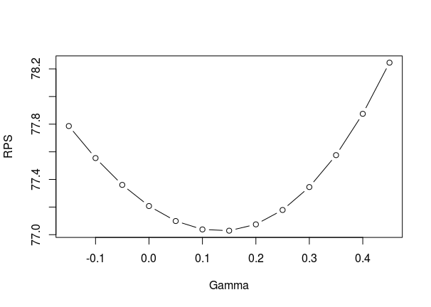
As you see I even tried some negative values of \(\gamma\), just in case. At least in this season the result agrees with the estimate \(\gamma = 0.1\) that Rue and Salvesen reported. In some of the later seasons that I checked the optimal \(\gamma\) varies somewhat. In some seasons it is almost 0, but then again in some others it is around 0.1. So at least for Premier league, using \(\gamma = 0.1\) seems reasonable.
Things are a bit different in Bundesliga. Here is the same kind of plot for the 2011-12 season:

As you see the optimal value here is around 0.25. In the other seasons I checked the optimal value were somewhere between 0.15 and 0.3. So the effect of over- and underestimating the opponent seem to be greater in the Bundesliga than in Premier League.
deltaAB = (attA + defA – attB – defB) / 2
Setting gamma = 2 eg. we get:
lambdaA = a + b + attB – defA
lambdaB = a + attA – defB
That means the attack team of the opponent is considered to score and the
defense of the own teams is considered to defend the team from scoring.
Does this make sense?
Actually without losing anything, but the model could equivalently modelled as
lambdaA = a + b + attA – defB + gamma * attB – gamma * defA.
lambdaB analog
I agree that looking at the model that way is helpful. You can then see clearly that the all four team-specific parameters in the game end up in the calculation of both expected goals. I think this explain why I had trouble estimating the model.
Its astonishing that positive gamma give better results. I would expect a negative team dependent gamma perform better.
The idea is, that in weak teams usually the attack players must help out the defense players. In strong teams the defense part is better and the attack can do their job in scoring.
BTW, the dixon coles model is not the best. It corrects also the 1:1 score which is ok. The 0:0 is off.
I think it migh be because a good team who plays againt a poor team might not let the best players play, giving perhaps the more ju ior player a chance, or something. I think there is an opportunity to find which situations to use the adjustment, and when to not use it.
I don’t know much about soccer, but math.
So that means a team like Real, Barcelona have substiture players which don’t have same equality? But if one of these top players have an insurary. That means they cannot replace him. Is this reasonable?
Well easy to figure out, just code a poisson model in Stan and test by loo. The smaller looic the better. It provide a function compare to two or more looic by their crossvalided standard error approximated by pareto distribution.
I see a flaw in your analysis . How does the time of the opening goal effect expectation of the other team fighting back in an individual league ? The common thought process that the team -1 goal , shoot and score more goals is rubbish if you actually look at a large number of leagues around the globe > I have automated historical data for > 1-1 and > 2-0 / 0-2 game state in 64 leagues given the time of the opening goal ( first half ) if you are interested
I am not sure I understand what the flaw is. I don’t model the scoring times, only the number of goals scored in total.
Cool stuff. I can imagine a few ways this effect occurs:
– Better teams resting a few of their best players against weaker teams. This is fairly rare in the English PL, but does occur at least when the league match is followed by important Champions League matches.
– The winning team substituting out a few key players when they are in a winning position, to rest them or give time to younger players. Usually this is only done when the result of the match is secure, but it’s likely to have some impact on the net goals, e.g. a 3-0 position might end up 3-1 when it otherwise could have been 4-0.
– More generally, the winning team ‘taking it easy’ when in that 3-0 position.
Although, with the last two, I’d think almost always a 3-0 scoreline would be above the original (uncorrected) predicted win margin, so that the winning team taking it easy would help the original model, and it wouldn’t need the correction. The first explanation is more convincing then, as teams can be ‘caught out’ and perform worse than they would be comfortable with in these situations.
To onkel zaharias’s point, I wonder if the effect you describe is already built in to the original model – because weaker teams on average generally play against stronger teams, so their attackers have to do more defending usually, and this is then captured by the model fitting the coefficients for attack and defence. Or maybe both (counteracting) effects are built in to some extent, and this gamma term is some sort of residual from the two, which improves the model by telling it when one of the two effects is relatively stronger than the other (in a match).
With regard to understanding better when the correction should be used, I’d be interested to see two breakdowns:
– Improvement from gamma as a function of deltaAB; i.e. does this effect only really occur when the very best teams are involved (large deltaAB)?
– Improvement from gamma in periods affected by and not affected by upcoming Champions League games (roughly, mid-September to December and mid-Feb to April, vs the rest)
Thank you for your great comment! I haven’t had the time to look more into this lately, but I think your questions are reasonable and worth pursuing. The reason I haven’t had the time is because I am working on an R package to fit models with this adjustment. I am not sure when it will be ready, but most features have been implemented and I am working on documentation etc. Stay tuned!