
Last fall I took a short introduction course in Bayesian modeling, and as part of the course we were going to analyze a data set of our own. I of course wanted to model football results. The inspiration came from a paper by Gianluca Baio and Marta A. Blangiardo Bayesian hierarchical model for the prediction of football results (link).
I used data from Premier League from 2012 and wanted to test the predictions on the last half of the 2012-23 season. With this data I fitted two models: One where the number of goals scored where modeled using th Poisson distribution, and one where I modeled the outcome directly (as home win, away win or draw) using an ordinal probit model. As predictors I used the teams as categorical predictors, meaning each team will be associated with two parameters.
The Poisson model was pretty much the same as the first and simplest model described in Baio and Blangiardo paper, but with slightly more informed priors. What makes this model interesting and different from the independent Poisson model I have written about before, apart from being estimated using Bayesian techniques, is that each match is not considered as two independent events when the parameters are estimated. Instead a correlation is implicitly modeled by specifying the priors in a smart way (see figure 1 in the paper, or here), thereby modeling the number of goals scored like a sort-of-bivariate Poisson.
Although I haven’t had time to look much into it yet, I should also mention that Baio and Blangiardo extended their model and used it this summer to model the World Cup. You can read more at Baio’s blog.
The ordinal probit model exploits the fact that the outcomes for a match can be thought to be on an ordinal scale, with a draw (D) considered to be ‘between’ a home win (H) and an away win (A). An ordinal probit model is in essence an ordinary linear regression model with a continuous response mu, that is coupled with a set of threshold parameters. For any value of mu the probabilities for any category is determined by the cumulative normal distribution and the threshold values. This is perhaps best explained with help from a figure:
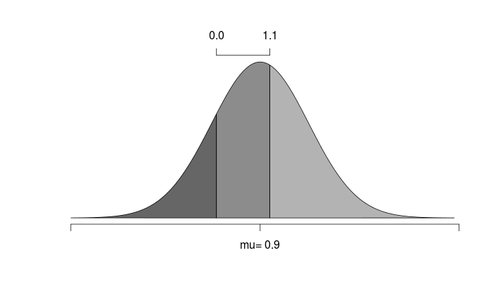
Here we see an example where the predicted outcome is 0.9, and the threshold parameters has been estimated to 0 and 1.1. The area under the curve is then the probability of the different outcomes.
To model the match outcomes I use a model inspired by the structure in the predictors as the Poisson model above. Since the outcomes are given as Away, Draw and Home, the home field advantage is not needed as a separate term. This is instead implicit in the coefficients for each team. This gives the coefficients a different interpretation from the above model. The two coefficients here can be interpreted as the ability when playing at home and the ability when playing away.
To get this model to work I had to set the constrains that the threshold separating Away and Draw were below the Draw-Home threshold. This implies that a good team would be expected to have a negative Away coefficient and a positive Home coefficient. Also, the intercept parameter had to be fixed to an arbitrary value (I used 2).
To estimate the parameters and make predictions I used JAGS trough the rjags package.
For both models, I used the most credible match outcome as the prediction. How well were the last half of the 2012-13 season predictions? The results are shown in the confusion table below.
Confusion matrix for Poisson model
| actual/predicted | A | D | H |
| A | 4 | 37 | 11 |
| D | 1 | 35 | 14 |
| H | 0 | 38 | 42 |
Confusion matrix for ordinal probit model
| actual/predicted | A | D | H |
| A | 19 | 0 | 33 |
| D | 13 | 0 | 37 |
| H | 10 | 0 | 70 |
The Poisson got the result right in 44.5% of the matches while the ordinal probit got right in 48.9%. This was better than the Poisson model, but it completely failed to even consider draw as an outcome. Ordinal probit, however, does seem to be able to predict away wins, which the Poisson model was poor at.
Here is the JAGS model specification for the ordinal probit model.
model {

  for( i in 1:Nmatches ) {

    pr[i, 1] <- phi( thetaAD - mu[i]  )
    pr[i, 2] <- max( 0 ,  phi( (thetaDH - mu[i]) ) - phi( (thetaAD - mu[i]) ) )
    pr[i, 3] <- 1 - phi( (thetaDH - mu[i]) )

    y[i] ~ dcat(pr[i, 1:3])

    mu[i] <- b0 + homePerf[teamh[i]] + awayPerf[teama[i]]
  }

  for (j in 1:Nteams){
    homePerf.p[j] ~ dnorm(muH, tauH)
    awayPerf.p[j] ~ dnorm(muA, tauA)

    #sum to zero constraint
    homePerf[j] <- homePerf.p[j] - mean(homePerf.p[])
    awayPerf[j] <- awayPerf.p[j] - mean(awayPerf.p[])
  }

  thetaAD ~ dnorm( 1.5 , 0.1 )
  thetaDH ~ dnorm( 2.5 , 0.1 )

  muH ~ dnorm(0, 0.01)
  tauH ~ dgamma(0.1, 0.1)

  muA ~ dnorm(0, 0.01)
  tauA ~ dgamma(0.1, 0.1)

  #predicting missing values
  predictions <- y[392:573]
}
And here is the R code I used to run the above model in JAGS.
library('rjags')
library('coda')

#load the data
dta <- read.csv('PL_1213.csv')

#Remove the match outcomes that should be predicted
to.predict <- 392:573 #this is row numbers
observed.results <- dta[to.predict, 'FTR']
dta[to.predict, 'FTR'] <- NA

#list that is given to JAGS
data.list <- list(
  teamh = as.numeric(dta[,'HomeTeam']),
  teama = as.numeric(dta[,'AwayTeam']),
  y = as.numeric(dta[, 'FTR']),
  Nmatches = dim(dta)[1],
  Nteams = length(unique(c(dta[,'HomeTeam'], dta[,'AwayTeam']))),
  b0 = 2 #fixed
)

#MCMC settings
parameters <- c('homePerf', 'awayPerf', 'thetaDH', 'thetaAD', 'predictions')
adapt <- 1000
burnin <- 1000
nchains <- 1
steps <- 15000
thinsteps <- 5

#Fit the model
#script name is a string with the file name where the JAGS script is.
jagsmodel <- jags.model(script.name, data=data.list, n.chains=nchains, n.adapt=adapt)
update(jagsmodel, n.iter=burnin)

samples <- coda.samples(jagsmodel, variable.names=parameters,
                        n.chains=nchains, thin=thinsteps,
                        n.iter=steps)

#Save the samples
save(samples, file='bayesProbit_20131030.RData')

#print summary
summary(samples)
Hi,
Can you share how to show the Confusion matrix in R for this samples?
Cou can use the table() function in R to create confusion tables. Suppose you have one vector with the actual results and one with your predictions:
results <- c('h', 'h', 'a', 'd', 'h', 'd', 'a')
predictions <-  c('h', 'd', 'a', 'a', 'a', 'h', 'd')
Pass these two to the table function:
table(results, predictions)could please show me how should I store the data, or where I can locate an filePL_1213.csv
You can download the data from http://www.football-data.co.uk/downloadm.php, and most scripts I post assumes the data is formated like those.
excuse me, I’m very new at this, engo problem jagsmodel <- jags.model (script.name, data = Data.List, n.chains = nchains, n.adapt = adapt)
update (jagsmodel, n.iter = burnin), I think it is because it is the first time that tranajo with jags
What sort of error messages do you get?
I don’t understand how you made the predictions. When I run summary(samples) it gives me a list called predictions all of whose entries are close to 2.
It’s been a while since I looked at this, but here’s my guess at whats going on. I code the three outcomes as 1, 2 and 3 (home, draw, and away). If you take the average (which is what the summary function presumably does), you should not be surprised that it is close to 2. Try instead counting the proportions of 1, 2 and 3’s in the MCMC samples. They should correspond to the probabilities of the three outcomes. Let me know if it doesn’t work, and I will take a closer look.
Counting the proportions will give me the probabilities, but then how am I supposed to predict the exact outcome of, say, the 224th match.
The prediction you get is what is called a probabalisticprediction. If you want a single outcome prediction, there are several options. The easiest thing to do is to select the outcome with highest probability as your prediction.
Hi, I am trying to implement this algorithm, and I am not sure if the results I am getting are correct.
For example in order to get the predicted value for the 80th game I do (I have 80 games which I need to predict):
mean(as.matrix(samples[,120,])
Is this correct or am I doing something wrong, since all the results I am getting are close to 2?
This is literally the same problem Raval had. Count the proportions of 1’s, 2’s and 3’s instead of averagning over them.