The Dixon-Coles approach to time-weighted Poisson regression

In the previous blog posts about predicting football results using Poisson regression I have mostly ignored the fact that the data points (ie matches) used to fit the models are gathered (played) at different time points.

In the 1997 Dixon and Coles paper where they described the bivariate adjustment for low scores they also discussed using weighted maximum likelihood to better make the parameter estimates reflect the current abilities of the teams, rather than as an average over the whole period you have data from.

Dixon and Coles propose to weight the games using a function so that games are down weighted exponentially by how long time it is since they were played. The function to determine the weight for a match played is

\( \phi(t) = exp(-\xi t) \)

where t is the time since the match was played, and \(\xi\) is a positive parameter that determines how much down-weighting should occur.

I have implemented this function in R, but I have done a slight modification from the one from the paper. Dixon and Coles uses “half weeks” as their time unit, but they do not describe in more detail what exactly they mean. They probably used Wednesday or Thursday as the day a new half-week starts, but I won’t bother implementing something like that. Instead I am just going to use days as the unit of time.

This function takes a vector of the match dates (data type Date) and computes the weights according to the current date and a value of \(\xi\). The currentDate argument lets you set the date to count from, with all dates after this will be given weight 0.

DCweights <- function(dates, currentDate=Sys.Date(), xi=0){
  datediffs <- dates - as.Date(currentDate)
  datediffs <- as.numeric(datediffs *-1)
  w <- exp(-1*xi*datediffs)
  w[datediffs <= 0] <- 0 #Future dates should have zero weights
  return(w)
}

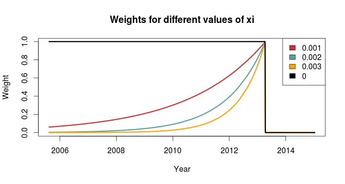
We can use this function to plot how the much weight the games in the past is given for different values of \(\xi\). Here we see that \(\xi = 0\) gives the same weight to all the matches. I have also set the currentDate as a day in April 2013 to illustrate how future dates are weighted 0.

WeightXi

To figure out the optimal value for \(\xi\) Dixon and Coles emulated a situation where they predicted the match results using only the match data prior to the match in question, and then optimizing for prediction ability. They don’t explain how exactly they did the optimizing, but I am not going to use the optim function to do this. Instead I am going to just try a lot of different values of \(\xi\), and go for the one that is best. The reason for this is that doing the prediction emulation takes some time, and using an optimizing algorithm will take an unpredictable amount of time.

I am not going to use the Dixon-Coles model here. Instead I am going for the independent Poisson model. Again, the reason is that I don’t want to use too much time on this.

To measure prediction ability, Dixon & Coles used the predictive log-likelihood (PLL). This is just the logarithm of the probabilities calculated by the model for the outcome that actually occurred, added together for all matches. This means that a greater PLL indicates that the actual outcomes was more probable according to the model, which is what we want.

I want to use an additional measure of prediction ability to complement the PLL: The ranked probability score (RPS). This is a measure of prediction error, and takes on values between 0 and 1, with 0 meaning perfect prediction. RPS measure takes into account the entire probability distribution for the three outcomes, not just the probability of the observed outcome. That means a high probability of a draw is considered less of an error that a high probability of away win, if the actual outcome was home win. This measure was popularized in football analytics by Anthony Constantinou in his paper Solving the Problem of Inadequate Scoring Rules for Assessing Probabilistic Football Forecast Models. You can find a link to a draft version of that paper on Constantinou’s website.

I used data from the 2005-06 season and onwards, and did predictions from January 2007 and up until the end of 2014. I also skipped the ten first match days at the beginning of each season to avoid problems with lack of data for the promoted teams. I did this for the top leagues in England, Germany, Netherlands and France. Here are optimal values of \(\xi\) according to the two prediction measurements:

PLL RPS
England 0.0018 0.0018
Germany 0.0023 0.0023
Netherlands 0.0019 0.0020
France 0.0019 0.0020

The RPS and PLL mostly agree, and where they disagree, it is only by one in the last decimal place.

Dixon & Coles found an optimal value of 0.0065 in their data (which were from the 1990s and included data from the top four English leagues and the FA cup), but they used half weeks instead of days as their time unit. Incidentally, if we divide their value by the number of days in a half week (3.5 days) we get 0.00186, about the same I got. The German league has the greatest optimum value, meaning historical data is of less importance when making predictions.

An interesting thing to do is to plot the predictive ability against different values of \(\xi\). Here are the PLL (adjusted to be between 0 and 1, with the optimum at 1) for England and Germany compared, with their optima indicated by the dashed vertical lines:

Prediction ability for values of Xi Engand Germany

I am not sure I want to interpret this plot too much, but it does seems like predictions for the German league are more robust to values of \(\xi\) greater than the optimum, as indicated by the slower decline in the graph, than the English league.

So here I have presented the values of \(\xi\) for the independent Poisson regression model, but will these values be the optimal for the Dixon & Coles model? Probably not, but I suspect there will be less variability between the two models than between the same model fitted for different leagues.

The Dixon-Coles model, part 4: A trick to speed up estimation

In the previous installments in this series on implementing the Dixon-Coles model I complained a bit about the time it took to estimate the parameters. In the original implementation in part 1 it took about 40 seconds. Now 40 seconds is not much to complain about, there are a whole lot of other models and algorithms that takes much much longer time to fit (for my master’s I had some computations that took several months). Still, I wanted to make a few improvements.

The approach I described in part 3 is quite acceptable, I think, especially since it takes less than a second to fit the model. But still, I wanted to make some improvements to my original implementation.

There are several reasons for the estimation procedure being slow. I used a general purpose optimizer instead of a tailor-made algorithm, and I didn’t provide the optimizer with a function of the derivative of the model likelihood function, nor the function defining the constraint. This means that the optimizer have to estimate the derivatives by doing a lot of evaluations of the two functions with slight changes in the parameters. The most important speed bump, however, is probably due to how I implemented the constraint that all the average of the attack parameters should equal 1.

The alabama package I used relied on a technique called Lagrange multipliers, which is a very general method for constrained optimization. Instead of relying on general constrained optimization procedures, there is a trick commonly used in linear models with sum-to-zero constrained categorical parameters that we also can use here.

There has been some discussion and confusion in the comments about how categorical variables are coded and how R presents the results of the glm function. A thorough discussion of this is best left for another time, but let me explain how the sum-to-zero constraint is implemented in linear models. We will fit the model with this constraint and then make some adjustments later on to get the correct average-is-one constraint.

The sum-to-zero constraint basically says that the sum of all the parameters for a categorical variable must equal to zero:

\( \sum_{i=1} \theta_i = 0 \)

If we for example have three levels, we can write out the equation like this:

\( \theta_1 + \theta_2 + \theta_3 = 0 \)

If we subtract \( \theta_3\) and multiply both sides of the equation by minus 1 we get

\( – \theta_1 – \theta_2 = \theta_3 \)

Notice how we can write one of the parameters as a simple linear function of the other parameters. We can use this result to construct the design matrix for the categorical variable, incorporating the sum-to-zero constraint (exactly which parameter or level we chose to be a function of the others doesn’t matter, the end results does not differ). Suppose we have the following observations of a three-level categorical variable:

\( \begin{bmatrix} A & A & B & B & C & C \end{bmatrix}^T \)

We can then construct the following design matrix:

\( \begin{bmatrix} 1 & 0 \\ 1 & 0 \\ 0 & 1 \\ 0 & 1 \\ -1 & -1 & \\ -1 & -1 & \end{bmatrix} \)

Notice that we only need two columns (i.e. two variables) to encode the three levels. Since the last parameter is a function of the two other it is redundant. Also notice how the observations in the two last rows, corresponding to the \(C\) observations, will influence the estimation of all the other parameters for this variable. When the two parameters are estimated, the last parameter can be obtained using the result from above relating the last parameter to all the other.

In the Dixon-Coles paper they used the constraint that the average of the attack parameters should be 1. This is not quite the same as the sum-to-zero constraint, but for prediction, it does not matter exactly which constraint we use. Anyway, I will explain later how we can fix this.

To use this trick in the Dixon-Coles implementation we need to make the following changes to our code from part 1. Obviously the first thing we need to change is how the design matrices in the DCmodelData function is computed. We need four matrices now, since the number of parameters estimated directly is different for the attack and defense parameters. Notice how I chose the last of team that appear last in the team.names vector. The teams get sorted alphabetically, so for the 2011-12 Premier League data this is is Wolves.

DCmodelData <- function(df){
  
  team.names <- unique(c(levels(df$HomeTeam), levels(df$AwayTeam)))
  
  # attack, with sum-to-zero constraint
  ## home
  hm.a <- model.matrix(~ HomeTeam - 1, data=df)
  hm.a[df$HomeTeam == team.names[length(team.names)], ] <- -1
  hm.a <- hm.a[,1:(length(team.names)-1)]
  
  # away
  am.a <- model.matrix(~ AwayTeam -1, data=df)
  am.a[df$AwayTeam == team.names[length(team.names)], ] <- -1
  am.a <- am.a[,1:(length(team.names)-1)]
  
  # defence, same as before 
  hm.d <- model.matrix(~ HomeTeam - 1, data=df)
  am.d <- model.matrix(~ AwayTeam -1, data=df)
  
  return(list(homeTeamDMa=hm.a, homeTeamDMd=hm.d,
    awayTeamDMa=am.a, awayTeamDMd=am.d,
    homeGoals=df$FTHG, awayGoals=df$FTAG,
    teams=team.names)) 
}

Some changes to the DCoptimFn function is also needed, so it properly handles the changes we made to the design matrices.

# I don't bother showing the rest of the function  
nteams <- length(DCm$teams)
attack.p <- matrix(params[3:(nteams+1)], ncol=1) #one column less
defence.p <- matrix(params[(nteams+2):length(params)], ncol=1) 
 
# need to multiply with the correct matrices
lambda <- exp(DCm$homeTeamDMa %*% attack.p + DCm$awayTeamDMd %*% defence.p + home.p)
mu <- exp(DCm$awayTeamDMa %*% attack.p + DCm$homeTeamDMd %*% defence.p)

We also need to make a the appropriate adjustments to the vectors with the initial parameter values, so that they have the correct lengths.

dcm <- DCmodelData(data)
nteams <- length(dcm$teams)

#initial parameter estimates
attack.params <- rep(.1, times=nteams-1) # one less parameter
defence.params <- rep(-0.8, times=nteams)
home.param <- 0.06
rho.init <- 0.03
par.inits <- c(home.param, rho.init, attack.params, defence.params)

#informative names
#skip the last team
names(par.inits) <- c('HOME', 'RHO', 
                      paste('Attack', dcm$teams[1:(nteams-1)], sep='.'),
                      paste('Defence', dcm$teams, sep='.'))

With these changes we can simply use the built-in optim function in R. There is no need for the DCattackConstr function anymore, or a third party package, since we built the constraint right into the design matrices.

res <- optim(par=par.inits, fn=DCoptimFn, DCm=dcm, method='BFGS')

This takes about 6-7 seconds on my laptop, a decent improvement to the 40 seconds it took before. If you take a look at the resulting parameter estimates in res$par you will see that the attack parameter for Wolves is missing. As I explained earlier, this parameter is easy to find. It is also easy to correct all the parameter estimates so that they become the same as if we had a mean-is-one constraint on the attack parameters. This is done by increasing the attack parameters by one, and decreasing the defense parameters by one. The reason it is that simple is that the sum-to-zero constraint is equivalent with a mean-is-zero constraint.

parameters <- res$par

#compute Wolves attack parameter
missing.attack <- sum(parameters[3:(nteams+1)]) * -1

#put it in the parameters vector
parameters <- c(parameters[1:(nteams+1)], missing.attack, parameters[(nteams+2):length(parameters)])
names(parameters)[nteams+2] <- paste('Attack.', dcm$teams[nteams], sep='')

#increase attack by one
parameters[3:(nteams+2)] <- parameters[3:(nteams+2)] + 1  

#decrease defence by one
parameters[(nteams+3):length(parameters)] <- parameters[(nteams+3):length(parameters)] - 1 

The Dixon-Coles model for predicting football matches in R (part 3)

About a moth ago Martin Eastwood of the pena.lt/y blog put up some slides from a talk he gave about predicting football results in R. He presented in detail the independent Poisson regression model, and how to implement it. He also briefly mentioned and showed the bivariate adjustments in the Dixon-Coles model. I was curious about how he had implemented it since I had just finished my own implementation. In the comments he said that he used a two-stage approach, first estimating the attack and defense parameters using the independent Poisson model, and then estimating the rho parameter by it self.

This method may be less accurate than fitting the complete model, but it will probably be more accurate than the independent Poisson model. It is without a doubt faster and easier to implement.

We start with loading the data, and then making a new data.frame that contains two rows per match, as described in my post about the independent Poisson model.

dta <- read.csv('FAPL1112.csv')

# Data formated for the independent model
# Store in new variable, we need the data in original format later
dta.indep <- data.frame(Team=as.factor(c(as.character(dta$HomeTeam),
                            as.character(dta$AwayTeam))),
                            Opponent=as.factor(c(as.character(dta$AwayTeam),
                            as.character(dta$HomeTeam))),
                            Goals=c(dta$FTHG, dta$FTAG),
                            Home=c(rep(1, dim(dta)[1]), rep(0, dim(dta)[1])))

Now fit the model:

m <- glm(Goals ~ Home + Team + Opponent, data=dta.indep, family=poisson())

Since we now have estimated the attack, defense and home parameters we can use the built-in functions in R to calculate the expected home and away scores (lambda and mu).

To calculate lambda and mu, we use the fitted function. I organized the data so that all the rows with the goals scored by the home team comes before all the rows with the goals by the away teams. Whats more, the match in the first row in the home team part corresponds to the match in the first row in the away team part, so it is easy to get the corresponding expectations correct.

expected <- fitted(m)
home.expected <- expected[1:nrow(dta)]
away.expected <- expected[(nrow(dta)+1):(nrow(dta)*2)]

To estimate the rho parameter we can use the tau and DClogLik function we defined in part 1. We just wrap it inside a function we pass to the built in optimizer in R:

DCoptimRhoFn <- function(par){
  rho <- par[1]
  DClogLik(dta$FTHG, dta$FTAG, home.expected, away.expected, rho)
}

res <- optim(par=c(0.1), fn=DCoptimRhoFn, control=list(fnscale=-1), method='BFGS')

The optimization finishes in an instant. As before we get the parameter values by looking at res$par. The estimated rho parameter is -0.126, which is reassuringly not that different from the -0.134 we got from the full model. This is is also about the same values Justin Worrall gets at his sportshacker.net blog.

To make predictions we can reuse most of the code from part 2. The only substantial difference is how we calculate the expected goals, which is a bit simpler this time:

# Expected goals home
lambda <- predict(m, data.frame(Home=1, Team='Bolton', Opponent='Blackburn'), type='response')

# Expected goals away
mu <- predict(m, data.frame(Home=0, Team='Blackburn', Opponent='Bolton'), type='response')

This two-stage approach is much faster and simpler. We don’t have to manually create the design matrices and use matrix algebra to calculate the expected scores. We also don’t have to write as much code to keep track of all the parameters. I haven’t really compared all the different models against each other, so I can’t say which one makes the best predictions, but my guess is that this two-stage approach gives results similar to the fully specified Dixon-Coles model.

The Dixon-Coles model for predicting football matches in R (part 2)

Part 1 ended with running the optimizer function to estimate the parameters in the model:

library(alabama)
res <- auglag(par=par.inits, fn=DCoptimFn, heq=DCattackConstr, DCm=dcm)

# Take a look at the parameters
res$par

In part 1 I fitted the model to data from the 2011-12 Premier League season. Now it’s time to use the model to make a prediction. As an example I will predict the result of Bolton playing at home against Blackburn.

The first thing we need to do is to calculate the mu and lambda parameters, which is (approximately anyway) the expected number of goals scored by the home and away team. To do this wee need to extract the correct parameters from the res$par vector. Recall that I in the last post gave the parameters informative names that consists of the team name prefixed by either Attack or Defence.
Also notice that I have to multiply the team parameters and then exponentiate the result to get the correct answer.

Update: For some reason I got the idea that the team parameters should be multiplied together, instead of added together, but I have now fixed the code and the results.

# Expected goals home
lambda <- exp(res$par['HOME'] + res$par['Attack.Bolton'] + res$par['Defence.Blackburn'])

# Expected goals away
mu <- exp(res$par['Attack.Blackburn'] + res$par['Defence.Bolton'])

We get that Bolton is expected to score 2.07 goals and Blackburn is expected to score 1.59 goals.

Since the model assumes dependencies between the number of goals scored by the two teams, it is insufficient to just plug the lambda and mu parameters into R’s built-in Poisson function to get the probabilities for the number of goals scored by the two teams. We also need to incorporate the adjustment for the low-scoring results as well. One strategy to do this is to first create a matrix based on the simple independent Poisson distributions:

maxgoal <- 6 # will be useful later
probability_matrix <- dpois(0:maxgoal, lambda) %*% t(dpois(0:maxgoal, mu))

The number of home goals follows the vertical axis and the away goals follow the horizontal.

Now we can use the estimated dependency parameter rho to create a 2-by-2 matrix with scaling factors, that is then element-wise multiplied with the top left elements of the matrix calculated above:

Update: Thanks to Mike who pointed out a mistake in this code.

scaling_matrix <- matrix(tau(c(0,1,0,1), c(0,0,1,1), lambda, mu, res$par['RHO']), nrow=2)
probability_matrix[1:2, 1:2] <- probability_matrix[1:2, 1:2] * scaling_matrix

With this matrix it is easy to calculate the probabilities for the three match outcomes:

HomeWinProbability <- sum(probability_matrix[lower.tri(probability_matrix)])
DrawProbability <- sum(diag(probability_matrix))
AwayWinProbability <- sum(probability_matrix[upper.tri(probability_matrix)])

This gives a probability of 0.49 for home win, 0.21 for draw and 0.29 for away win.

Calculating the probabilities for the different goal differences is a bit trickier. The probabilities for each goal difference can be found by adding up the numbers on the diagonals, with the sum of the main diagonal being the probability of a draw.

awayG <- numeric(maxgoal)
 for (gg in 2:maxgoal){
   awayG[gg-1] <- sum(diag(probability_matrix[,gg:(maxgoal+1)]))
 }
awayG[maxgoal] <- probability_matrix[1,(maxgoal+1)]

homeG <- numeric(maxgoal)
  for (gg in 2:maxgoal){
    homeG[gg-1] <- sum(diag(probability_matrix[gg:(maxgoal+1),]))
  }
homeG[maxgoal] <- probability_matrix[(maxgoal+1),1]

goaldiffs <- c(rev(awayG), sum(diag(probability_matrix)), homeG)
names(goaldiffs) <- -maxgoal:maxgoal

It is always nice to plot the probability distribution:

DCBoltonBlackburn

We can also see compare this distribution with the distribution without the Dixon-Coles adjustment (i.e. the goals scored by the two teams are independent):

DCboltonBlackburn2

As expected, we see that the adjustment gives higher probability for draw, and lower probabilities for goal differences of one goal.

The Dixon-Coles model for predicting football matches in R (part 1)

Please have a look at the improved code for this model that I have posted here.

When it comes to Poisson regression models for football results, the 1997 paper Modelling Association Football Scores and Inefficiencies in the Football Betting Market (pdf) by Dixon and Coles is often mentioned. In this paper the authors describe an improvement of the independent goals model. The improvement consists of modeling a dependence between the probabilities for the number of goals less than 2 for both teams. They also improve the model by incorporating a time perspective, so that matches played a long time a go does not have as much influence on the parameter estimates.

The model by Dixon and Coles is not as easy to fit as the independent Poisson model I have described earlier. There is no built-in function in R that can estimate it’s parameters, and the authors provide little details about how to implement it. Mostly as an exercise, I have implemented the model in R, but without the time down-weighting scheme.

The estimating procedure uses a technique called maximum likelihood. This is perhaps the most commonly used method for estimating parameters in statistical models. The way it works is that you specify a way to calculate the likelihood of your data for a given set of parameters, and then you need to find the set of parameters that gives the highest possible likelihood of your data. The independent Poisson model is also fitted using a maximum likelihood method. The difference here is that the likelihood used by Dixon and Coles is non-standard.

The model is pretty much similar to other regression models I have discussed. Each team has an attack and a defense parameter, and from a function of these the expected number of goals for each team in a match is calculated. For the rest of this post I am going to assume you have read the paper. There is a link to it in the first paragraph.

The most obvious thing we have to do is to implement the function referred to by the greek letter Tau. This is the function that, dependent on the Rho parameter, computes the degree in which the probabilities for the low scoring goals changes.

tau <- Vectorize(function(xx, yy, lambda, mu, rho){
  if (xx == 0 & yy == 0){return(1 - (lambda*mu*rho))
  } else if (xx == 0 & yy == 1){return(1 + (lambda*rho))
  } else if (xx == 1 & yy == 0){return(1 + (mu*rho))
  } else if (xx == 1 & yy == 1){return(1 - rho)
  } else {return(1)}
})

We can now make a function for the likelihood of the data. A common trick when implementing likelihood functions is to use the log-likelihood instead. The reason is that when the probabilities for each data point for a given set of parameters are multiplied together, they will be too small for the computer to handle. When the probabilities are log-transformed you can instead just add them together.

What this function does is that it takes the vectors of mu (expected home goals) and lambda (expected away goals), Rho, and the vectors of observed home and away goals, and computes the log-likelihood for all the data.

DClogLik <- function(y1, y2, lambda, mu, rho=0){
  #rho=0, independence
  #y1: home goals
  #y2: away goals
  sum(log(tau(y1, y2, lambda, mu, rho)) + log(dpois(y1, lambda)) + log(dpois(y2, mu)))
}

The team specific attack and defense parameters are not included in the log-likelihood function. Neither is the code that calculates the expected number of goals for each team in a match (lambda and mu). Before we can calculate these for each match, we need to do some data wrangling. Here is a function that takes a data.frame formated like the data from football-data.co.uk, and returns a list with design matrices and vectors with the match results.

DCmodelData <- function(df){

  hm <- model.matrix(~ HomeTeam - 1, data=df, contrasts.arg=list(HomeTeam='contr.treatment'))
  am <- model.matrix(~ AwayTeam -1, data=df)
  
  team.names <- unique(c(levels(df$HomeTeam), levels(df$AwayTeam)))
  
  return(list(
    homeTeamDM=hm,
    awayTeamDM=am,
    homeGoals=df$FTHG,
    awayGoals=df$FTAG,
    teams=team.names
    )) 
}

Now we create a function that calculates the log-likelihod from a set of parameters and the data we have. First it calculates the values for lambda and mu for each match, then it passes these and the number of goals scored in each match to the log-likelihood function.

This function needs to be written in such a way that it can be used by another function that will find the parameters that maximizes the log-likelihood. First, all the parameters needs to be given to a single argument in the form of a vector (the params argument). Also, the log-likelihood is multiplied by -1, since the optimization function we are going to use only minimizes, but we want to maximize.

DCoptimFn <- function(params, DCm){

  home.p <- params[1]
  rho.p <- params[2]
  
  nteams <- length(DCm$teams)
  attack.p <- matrix(params[3:(nteams+2)], ncol=1)
  defence.p <- matrix(params[(nteams+3):length(params)], ncol=1)
  
  lambda <- exp(DCm$homeTeamDM %*% attack.p + DCm$awayTeamDM %*% defence.p + home.p)
  mu <- exp(DCm$awayTeamDM %*% attack.p + DCm$homeTeamDM %*% defence.p)
  
  return(
    DClogLik(y1=DCm$homeGoals, y2=DCm$awayGoals, lambda, mu, rho.p) * -1
    )
}

One more thing we need before we start optimizing is a function that helps the optimizer handle the constraint that all the attack parameters must sum to 1. If this constraint isn’t given, it will be impossible to find a unique set of parameters that maximizes the likelihood.

DCattackConstr <- function(params, DCm, ...){
  nteams <- length(DCm$teams)
  attack.p <- matrix(params[3:(nteams+2)], ncol=1)
  return((sum(attack.p) / nteams) - 1)
}

Now we are finally ready to find the parameters that maximizes the likelihood based on our data. First, load the data (in this case data from the 2011-12 premier league), and properly handle it with our DCmodelData function:

dta <- read.csv('FAPL1112.csv')
dcm <- DCmodelData(dta)

Now we need to give a set of initial estimates of our parameters. It is not so important what specific values these are, but should preferably be in the same order of magnitude as what we think the estimated parameters should be. I set all attack parameters to 0.1 and all defense parameters to -0.8.

#initial parameter estimates
attack.params <- rep(.01, times=nlevels(dta$HomeTeam))
defence.params <- rep(-0.08, times=nlevels(dta$HomeTeam))
home.param <- 0.06
rho.init <- 0.03
par.inits <- c(home.param, rho.init, attack.params, defence.params)
#it is also usefull to give the parameters some informative names
names(par.inits) <- c('HOME', 'RHO', paste('Attack', dcm$teams, sep='.'), paste('Defence', dcm$teams, sep='.'))

To optimize with equality constraints (all attack parameters must sum to 1) we can use the auglag function in the alabama package. This takes about 40 seconds to run on my laptop, much longer than the independent Poisson model fitted with the built in glm function. This is because the auglag function uses some general purpose algorithms that can work with a whole range of home-made functions, while the glm function is implemented with a specific set of models in mind.

library(alabama)
res <- auglag(par=par.inits, fn=DCoptimFn, heq=DCattackConstr, DCm=dcm)

Voilà! Now the parameters can be found by the command res$par. In a follow-up post I will show how we can use the model to make prediction of match outcomes.

Team Attack Defence
Arsenal 1.37 -0.91
Aston Villa 0.69 -0.85
Blackburn 0.94 -0.47
Bolton 0.92 -0.48
Chelsea 1.23 -0.97
Everton 0.94 -1.15
Fulham 0.93 -0.89
Liverpool 0.89 -1.13
Man City 1.56 -1.43
Man United 1.52 -1.31
Newcastle 1.10 -0.88
Norwich 1.02 -0.62
QPR 0.82 -0.65
Stoke 0.64 -0.87
Sunderland 0.86 -0.99
Swansea 0.85 -0.89
Tottenham 1.24 -1.09
West Brom 0.86 -0.88
Wigan 0.81 -0.71
Wolves 0.79 -0.42
Home 0.27
Rho -0.13

Two Bayesian regression models for football results

Last fall I took a short introduction course in Bayesian modeling, and as part of the course we were going to analyze a data set of our own. I of course wanted to model football results. The inspiration came from a paper by Gianluca Baio and Marta A. Blangiardo Bayesian hierarchical model for the prediction of football results (link).

I used data from Premier League from 2012 and wanted to test the predictions on the last half of the 2012-23 season. With this data I fitted two models: One where the number of goals scored where modeled using th Poisson distribution, and one where I modeled the outcome directly (as home win, away win or draw) using an ordinal probit model. As predictors I used the teams as categorical predictors, meaning each team will be associated with two parameters.

The Poisson model was pretty much the same as the first and simplest model described in Baio and Blangiardo paper, but with slightly more informed priors. What makes this model interesting and different from the independent Poisson model I have written about before, apart from being estimated using Bayesian techniques, is that each match is not considered as two independent events when the parameters are estimated. Instead a correlation is implicitly modeled by specifying the priors in a smart way (see figure 1 in the paper, or here), thereby modeling the number of goals scored like a sort-of-bivariate Poisson.

Although I haven’t had time to look much into it yet, I should also mention that Baio and Blangiardo extended their model and used it this summer to model the World Cup. You can read more at Baio’s blog.

The ordinal probit model exploits the fact that the outcomes for a match can be thought to be on an ordinal scale, with a draw (D) considered to be ‘between’ a home win (H) and an away win (A). An ordinal probit model is in essence an ordinary linear regression model with a continuous response mu, that is coupled with a set of threshold parameters. For any value of mu the probabilities for any category is determined by the cumulative normal distribution and the threshold values. This is perhaps best explained with help from a figure:

probit_treshold_example

Here we see an example where the predicted outcome is 0.9, and the threshold parameters has been estimated to 0 and 1.1. The area under the curve is then the probability of the different outcomes.

To model the match outcomes I use a model inspired by the structure in the predictors as the Poisson model above. Since the outcomes are given as Away, Draw and Home, the home field advantage is not needed as a separate term. This is instead implicit in the coefficients for each team. This gives the coefficients a different interpretation from the above model. The two coefficients here can be interpreted as the ability when playing at home and the ability when playing away.

To get this model to work I had to set the constrains that the threshold separating Away and Draw were below the Draw-Home threshold. This implies that a good team would be expected to have a negative Away coefficient and a positive Home coefficient. Also, the intercept parameter had to be fixed to an arbitrary value (I used 2).

To estimate the parameters and make predictions I used JAGS trough the rjags package.

For both models, I used the most credible match outcome as the prediction. How well were the last half of the 2012-13 season predictions? The results are shown in the confusion table below.

Confusion matrix for Poisson model

actual/predicted A D H
A 4 37 11
D 1 35 14
H 0 38 42

Confusion matrix for ordinal probit model

actual/predicted A D H
A 19 0 33
D 13 0 37
H 10 0 70

The Poisson got the result right in 44.5% of the matches while the ordinal probit got right in 48.9%. This was better than the Poisson model, but it completely failed to even consider draw as an outcome. Ordinal probit, however, does seem to be able to predict away wins, which the Poisson model was poor at.

Here is the JAGS model specification for the ordinal probit model.

model {

  for( i in 1:Nmatches ) {

    pr[i, 1] <- phi( thetaAD - mu[i]  )
    pr[i, 2] <- max( 0 ,  phi( (thetaDH - mu[i]) ) - phi( (thetaAD - mu[i]) ) )
    pr[i, 3] <- 1 - phi( (thetaDH - mu[i]) )

    y[i] ~ dcat(pr[i, 1:3])

    mu[i] <- b0 + homePerf[teamh[i]] + awayPerf[teama[i]]
  }

  for (j in 1:Nteams){
    homePerf.p[j] ~ dnorm(muH, tauH)
    awayPerf.p[j] ~ dnorm(muA, tauA)

    #sum to zero constraint
    homePerf[j] <- homePerf.p[j] - mean(homePerf.p[])
    awayPerf[j] <- awayPerf.p[j] - mean(awayPerf.p[])
  }

  thetaAD ~ dnorm( 1.5 , 0.1 )
  thetaDH ~ dnorm( 2.5 , 0.1 )

  muH ~ dnorm(0, 0.01)
  tauH ~ dgamma(0.1, 0.1)

  muA ~ dnorm(0, 0.01)
  tauA ~ dgamma(0.1, 0.1)

  #predicting missing values
  predictions <- y[392:573]
}

And here is the R code I used to run the above model in JAGS.

library('rjags')
library('coda')

#load the data
dta <- read.csv('PL_1213.csv')

#Remove the match outcomes that should be predicted
to.predict <- 392:573 #this is row numbers
observed.results <- dta[to.predict, 'FTR']
dta[to.predict, 'FTR'] <- NA

#list that is given to JAGS
data.list <- list(
  teamh = as.numeric(dta[,'HomeTeam']),
  teama = as.numeric(dta[,'AwayTeam']),
  y = as.numeric(dta[, 'FTR']),
  Nmatches = dim(dta)[1],
  Nteams = length(unique(c(dta[,'HomeTeam'], dta[,'AwayTeam']))),
  b0 = 2 #fixed
)

#MCMC settings
parameters <- c('homePerf', 'awayPerf', 'thetaDH', 'thetaAD', 'predictions')
adapt <- 1000
burnin <- 1000
nchains <- 1
steps <- 15000
thinsteps <- 5

#Fit the model
#script name is a string with the file name where the JAGS script is.
jagsmodel <- jags.model(script.name, data=data.list, n.chains=nchains, n.adapt=adapt)
update(jagsmodel, n.iter=burnin)

samples <- coda.samples(jagsmodel, variable.names=parameters, 
                        n.chains=nchains, thin=thinsteps,
                        n.iter=steps)

#Save the samples
save(samples, file='bayesProbit_20131030.RData')

#print summary
summary(samples)

Predicting football results with Adaptive Boosting

Adaptive Boosting, usually referred to by the abbreviation AdaBoost, is perhaps the best general machine learning method around for classification. It is what’s called a meta-algorithm, since it relies on other algorithms to do the actual prediction. What AdaBoost does is combining a large number of such algorithms in a smart way: First a classification algorithm is trained, or fitted, or its parameters are estimated, to the data. The data points that the algorithm misclassifies are then given more weight as the algorithm is trained again. This procedure is repeated a large number of times (perhaps many thousand times). When making predictions based on a new set of data, each of the fitted algorithms predict the new response value, and a the most commonly predicted value is then considered the overall prediction. Of course there are more details surrounding the AdaBoost than this brief summary. I can recommend the book The Elements of Statistical Learning by Hasite, Tibshirani and Friedman for a good introduction to AdaBoost, and machine learning in general.

Although any classification algorithm can be used with AdaBoost, it is most commonly used with decision trees. Decision trees are intuitive models that make predictions based on a combination of simple rules. These rules are usually of the form “if predictor variable x is greater than a value y, then do this, if not, do that”. By “do this” and “do that” I mean continue to a different rule of the same form, or make a prediction. This cascade of different rules can be visualized with a chart that looks sort of like a tree, hence the tree metaphor in the name. Of course Wikipedia has an article, but The Elements of Statistical Learning has a nice chapter about trees too.

In this post I am going to use decision trees and AdaBoost to predict the results of football matches. As features, or predictors I am going to use the published odds from different betting companies, which is available from football-data.co.uk. I am going to use data from the 2012-13 and first half of the 2013-14 season of the English Premier League to train the model, and then I am going to predict the remaining matches from the 2013-14 season.

Implementing the algorithms by myself would of course take a lot of time, but luckily they are available trough the excellent Python scikit-learn package. This package contains lots of machine learning algorithms plus excellent documentation with a lot of examples. I am also going to use the pandas package for loading the data.

import numpy as np
import pandas as pd

dta_fapl2012_2013 = pd.read_csv('FAPL_2012_2013_2.csv', parse_dates=[1])
dta_fapl2013_2014 = pd.read_csv('FAPL_2013-2014.csv', parse_dates=[1])

dta = pd.concat([dta_fapl2012_2013, dta_fapl2013_2014], axis=0, ignore_index=True)

#Find the row numbers that should be used for training and testing.
train_idx = np.array(dta.Date < '2014-01-01')
test_idx = np.array(dta.Date >= '2014-01-01')

#Arrays where the match results are stored in
results_train = np.array(dta.FTR[train_idx])
results_test = np.array(dta.FTR[test_idx])

Next we need to decide which columns we want to use as predictors. I wrote earlier that I wanted to use the odds for the different outcomes. Asian handicap odds could be included as well, but to keep things simple I am not doing this now.

feature_columns = ['B365H', 'B365D', 'B365A', 'BWH', 'BWD', 'BWA', 'IWH',
					'IWD', 'IWA','LBH', 'LBD', 'LBA', 'PSH', 'PSD', 'PSA',
					'SOH', 'SOD', 'SOA', 'SBH', 'SBD', 'SBA', 'SJH', 'SJD',
					'SJA', 'SYH', 'SYD','SYA', 'VCH', 'VCD', 'VCA', 'WHH',
					'WHD', 'WHA']

For some bookmakers the odds for certain matches is missing. In this data this is not much of a problem, but it could be worse in other data. Missing data is a problem because the algorithms will not work when some values are missing. Instead of removing the matches where this is the case we can instead guess the value that is missing. As a rule of thumb we can say that an approximate value for some variables of an observation is often better than dropping the observation completely. This is called imputation and scikit-learn comes with functionality for doing this for us.

The strategy I am using here is to fill inn the missing values by the mean of the odds for the same outcome. For example if the odds for home win from one bookmaker is missing, our guess of this odds is going to be the average of the odds for home win from the other bookmakers for that match. Doing this demands some more work since we have to split the data matrix in three.

from sklearn.preprocessing import Imputer

#Column numbers for odds for the three outcomes 
cidx_home = [i for i, col in enumerate(dta.columns) if col[-1] in 'H' and col in feature_columns]
cidx_draw = [i for i, col in enumerate(dta.columns) if col[-1] in 'D' and col in feature_columns]
cidx_away = [i for i, col in enumerate(dta.columns) if col[-1] in 'A' and col in feature_columns]

#The three feature matrices for training
feature_train_home = dta.ix[train_idx, cidx_home].as_matrix()
feature_train_draw = dta.ix[train_idx, cidx_draw].as_matrix()
feature_train_away = dta.ix[train_idx, cidx_away].as_matrix()

#The three feature matrices for testing
feature_test_home = dta.ix[test_idx, cidx_home].as_matrix()
feature_test_draw = dta.ix[test_idx, cidx_draw].as_matrix()
feature_test_away = dta.ix[test_idx, cidx_away].as_matrix()

train_arrays = [feature_train_home, feature_train_draw,
				feature_train_away]
									
test_arrays = [feature_test_home, feature_test_draw,
				feature_test_away]

imputed_training_matrices = []
imputed_test_matrices = []

for idx, farray in enumerate(train_arrays):
	imp = Imputer(strategy='mean', axis=1) #0: column, 1:rows
	farray = imp.fit_transform(farray)
	test_arrays[idx] = imp.fit_transform(test_arrays[idx])
	
	imputed_training_matrices.append(farray)
	imputed_test_matrices.append(test_arrays[idx])

#merge the imputed arrays
feature_train = np.concatenate(imputed_training_matrices, axis=1)
feature_test = np.concatenate(imputed_test_matrices, axis=1)

Now we are finally ready to use the data to train the algorithm. First an AdaBoostClassifier object is created, and here we need to give supply a set of arguments for it to work properly. The first argument is classification algoritm to use, which is the DecisionTreeClassifier algorithm. I have chosen to supply this algorithms with the max_dept=3 argument, which constrains the training algorithm to not apply more than three rules before making a prediction.

The n_estimators argument tells the algorithm how many decision trees it should fit, and the learning_rate argument tells the algorithm how much the misclassified matches are going to be up-weighted in the next round of decision three fitting. These two values are usually something that you can experiment with since there is no definite rule on how these should be set. The rule of thumb is that the lower the learning rate is, the more estimators you neeed.

The last argument, random_state, is something that should be given if you want to reproduce the model fitting. If this is not specified you will end up with slightly different trained algroithm each time you fit them. See this question on Stack Overflow for an explanation.

At last the algorithm is fitted using the fit() method, which is supplied with the odds and match results.

from sklearn.ensemble import AdaBoostClassifier
from sklearn.tree import DecisionTreeClassifier

adb = AdaBoostClassifier(
    DecisionTreeClassifier(max_depth=3),
    n_estimators=1000,
    learning_rate=0.4, random_state=42)

adb = adb.fit(feature_train, results_train)

We can now see how well the trained algorithm fits the training data.

import sklearn.metrics as skm

training_pred = adb.predict(feature_train)
print skm.confusion_matrix(list(training_pred), list(results_train))

This is the resulting confusion matrix:

Away Draw Home
Away 164 1 0
Draw 1 152 0
Home 0 0 152

We see that only two matches in the training data is misclassified, one away win which were predicted to be a draw and one draw that was predicted to be an away win. Normally with such a good fit we should be wary of overfitting and poor predictive power on new data.

Let’s try to predict the outcome of the Premier League matches from January to May 2014:

test_pred = adb.predict(feature_test)
print skm.confusion_matrix(list(test_pred), list(results_test)) 
Away Draw Home
Away 31 19 12
Draw 13 10 22
Home 20 14 59

It successfully predicted the right match outcome in a bit over half of the matches.

The R code for the home field advantage and traveling distance analysis.

I was asked in the comments on my Does traveling distance influence home field advantage? to provide the R code I used, because Klemens of the rationalsoccer blog wanted to do the analysis on some of his own data. I have refactored it a bit to make it easier to use.

First load the data with the coordinates I posted last year.

dta.stadiums <- read.csv('stadiums.csv')

I also assume you have data formated like the data from football-data.co.uk in a data frame called dta.matches.

First wee need a way to calculate the distance (in kilometers) between the two coordinates. This is a function that does that.

coordinate.distance <- function(lat1, long1, lat2, long2, radius=6371){
  #Calculates the distance between two WGS84 coordinates.
  #
  #http://en.wikipedia.org/wiki/Haversine_formula
  #http://www.movable-type.co.uk/scripts/gis-faq-5.1.html
  dlat <- (lat2 * (pi/180)) - (lat1 * (pi/180))
  dlong <- (long2 * (pi/180)) - (long1 * (pi/180))
  h <- (sin((dlat)/2))^2 + cos((lat1 * (pi/180)))*cos((lat2 * (pi/180))) * ((sin((dlong)/2))^2)
  c <- 2 * pmin(1, asin(sqrt(h)))
  d <- radius * c
  return(d)
}

Next, we need to find the coordinates where each match is played, and the coordinates for where the visting team comes from. Then the traveling distance for each match is calculated and put into the Distance column of dta.matches.

coord.home <- dta.stadiums[match(dta.matches$HomeTeam, dta.stadiums$FDCOUK),
                           c('Latitude', 'Longitude')]
coord.away <- dta.stadiums[match(dta.matches$AwayTeam, dta.stadiums$FDCOUK),
                           c('Latitude', 'Longitude')]

dta.matches$Distance <- coordinate.distance(coord.home$Latitude, coord.home$Longitude,
                                            coord.away$Latitude, coord.away$Longitude)

Here are two functions that is needed to calculate the home field advantage per match. The avgerage.gd function takes a data frame as an argument and computes the average goal difference for each team. The result should be passed to the matchwise.hfa function to calculate the the home field advantage per match.

avgerage.gd <- function(dta){
  #Calculates the average goal difference for each team.
  
  all.teams <- unique(c(levels(dta$HomeTeam), levels(dta$AwayTeam)))
  average.goal.diff <- numeric(length(all.teams))
  names(average.goal.diff) <- all.teams
  for (t in all.teams){
    idxh <- which(dta$HomeTeam == t)
    goals.for.home <- dta[idxh, 'FTHG']
    goals.against.home <- dta[idxh, 'FTAG']
    
    idxa <- which(dta$AwayTeam == t)
    goals.for.away <- dta[idxa, 'FTAG']  
    goals.against.away <- dta[idxa, 'FTHG']
    
    n.matches <- length(idxh) + length(idxa)
    total.goal.difference <- sum(goals.for.home) + sum(goals.for.away) - sum(goals.against.home) - sum(goals.against.away)
    
    average.goal.diff[t] <- total.goal.difference / n.matches
  }
  return(average.goal.diff)
}


matchwise.hfa <- function(dta, avg.goaldiff){
  #Calculates the matchwise home field advantage based on the average goal
  #difference for each team.
  
  n.matches <- dim(dta)[1]
  hfa <- numeric(n.matches)
  for (idx in 1:n.matches){
    hometeam.avg <- avg.goaldiff[dta[idx,'HomeTeam']]
    awayteam.avg <- avg.goaldiff[dta[idx,'AwayTeam']]
    expected.goal.diff <- hometeam.avg - awayteam.avg
    observed.goal.diff <- dta[idx,'FTHG'] - dta[idx,'FTAG']
    hfa[idx] <- observed.goal.diff - expected.goal.diff
  }
  return(hfa)
}

In my analysis I used data from several seasons, and the average goal difference for each team was calculated per season. Assuming you have added a Season column to dta.matches that is a factor indicating which season the match is from, this piece of code calculates the home field advantage per match based on the seasonwise average goal differences for each team (puh!). The home field advantage is out into the new column HFA.

dta.matches$HFA <- numeric(dim(dta.matches)[1])
seasons <- levels(dta.matches$Season)

for (i in 1:length(seasons)){
  season.l <- dta.matches$Season == seasons[i]
  h <- matchwise.hfa(dta.matches[season.l,], avgerage.gd(dta.matches[season.l,]))
  dta.matches$HFA[season.l] <- h
}

At last we can do the linear regression and make a nice little plot.

m <- lm(HFA ~ Distance, data=dta.matches)
summary(m)

plot(dta.matches$Distance, dta.matches$HFA, xlab='Distance (km)', ylab='Difference from expected goals', main='Home field advantage vs traveling distance')
abline(m, col='red')

The minimum violations ranking method

One informative benchmark when ranking and rating sports teams is how many times the ranking has been violated. A ranking violation occurs when a team beats a higher ranked team. Ideally no violations would occur, but in practice this rarely happens. In many cases it is unavoidable, for example in this three team competition: Team A beats team B, team B beats team C, and team C beats team A. In this case, for any of the 6 possible rankings of these three teams at least one violation would occur.

Inspired by this, one could try to construct a ranking with as few violations as possible. A minimum violations ranking (MVR), as it is called. The idea is simple and intuitive, and has been put to use in ranking American college sport teams. The MinV ranking by Jay Coleman is one example.

MV rankings have some other nice properties other than being just an intuitive measure. A MV ranking is the best ranking in terms of backwards predictions. It can also be a method for combining several other rankings, by using the other rankings as the data.

Despite this, I don’t think MV rankings are that useful in the context of football. The main reason for this is that football has a large number of draws and as far as I can tell, a draw has no influence on a MV ranking. A draw is therefore equivalent with no game at all and provides no information.

MV rankings also has another problem. In many cases there can be several rankings that satisfies the MV criterion. This of course depends on the data, but it seems nevertheless to be quite common, such as in the small example above.

Unfortunately, I have not found any software packages that can find a MV ranking. One algorithm is described in this paper (paywall), but I haven’t tried to implemented it myself. Most other MVR methods I have seen seem to be based on defining a set of mathematical constraints and then letting some optimization software search for solutions. See this paper for an example.

Does traveling distance influence home field advantage?

A couple of weeks ago I posted a data set with the location of the stadiums for many of the football teams in Europe. One thing I wanted to use the dataset for was to see if the traveling distance between two teams (as measured by the distance between the two team’s home stadium) influenced home field advantage.

To calculate the home field advantage for each match i did the following: For each team, the average goal difference during the season are calculated (goals scored minus goals conceded divided by the number of matches). Then the expected goal difference for a match is the difference between the average goal differences (home minus away). The home field advantage is then the observed goal difference minus the expected goal difference.

In the 2012-13 Premier League season, for example, Chelsea scored 75 goals and conceded 39 goals in total. Everton scored 55 and conceded 40 goals. Both teams played 38 matches during the season. On average Chelsea had a goal difference of per match of 0.947 and Everton’s average were 0.395. With Chelsea meeting Everton at home the expected goal difference is 0.947 – 0.395 = 0.553. The actual outcome for this match was 2-1, a goal difference of 1. The home field advantage for this match is then 1 – 0.553 = 0.447.

Using data from the 2011-12 and 2012-13 seasons from the top divisions from Spain, France Germany, and the 2012-13 from England I used the stadium coordinates to calculate the traveling distance for the visiting team and the home field advantage. Plotting these two against each other, and drawing the least squares line gives this:

hfadistance

There is a great deal of noise in this plot, to put it mildly. The slope of the red line is 0.00006039. This is the estimated increase in number of goals the home team scores for each kilometer the away team has traveled. This is not significantly different from 0 (p-value = 0.646). The intercept, where the red line crosses the vertical axis is 0.4, meaning that the home team is estimated to score 0.4 more goals than expected, if the opposing team has traveled 0 kilometers. This is highly significant (p-value = 1.71e-11).

To be honest, I am a bit surprised to see such a clear lack of effect of traveling distance. I did not expect a particularly strong, or even very significant effect, but I had hoped to see at least a hint at something. Perhaps one reason for the lack of effect is that traveling distance is not necessarily the same as traveling time as longer distances may be covered by air, making them comparable to shorter travels by land.

It should be kept in mind that these results should only apply to the leagues included in the data. It could be that traveling distance could have a significant effect on longer distances, for example in international competitions such as the Champions League or between national teams.