Tuning the Elo ratings: Initial ratings and inter-league matches

In the last post I discussed how to tune the Elo ratings to make the ratings have the best predictive power by finding the optimal update factor (the K-factor) and adjustment for home field advantage. One thing I only mentioned, but did not go into detail about, was that the teams initial ratings will influence this tuning. In this post I will show how we can find good initial ratings that also will mitigate some other problems associated with Elo ratings.

As far as I can tell, setting the initial ratings does not seem to be much discussed. The Elo system updates the ratings by looking at the difference between the actual results and the results predicted by the rating difference between the two opposing teams. To get this to work in the earliest games in the data, you need to supply some initial ratings.

It is possible to set the initial ratings by hand, using your knowledge about the strengths of the different players and teams. This strategy is however difficult to use in practice, since you may not have that knowledge, which in turn would give incorrect ratings. This task would also become more difficult the more teams and players are in your data. An automatic way to get the initial ratings is of course preferable.

The only automatic way to set the initial ratings I have seen is to set all ratings to be equal. This is what they do at FiveThirtyEight. This simple strategy is obviously not optimal. It is a bit far fetched to assume that all teams are equally good at the beginning of your data, even if you could argue that you don’t really know any better. If you have a lot of data going back a long time, then only the earliest period of your ratings will be unrealistic. After a while the ratings will become more realistic and better reflect the true strengths of the teams.

The unrealistic ratings for the earliest data may also cause a problem if you use this to find the optimal K-factor. In Elo ratings the K-factor is a parameter that determines how much new games will influence the ratings. A larger K-factor makes the ratings change a lot after a new game, while a low K-factor will make the ratings change only a little after each new game. If you are trying to make a rating system with good prediction ability and use the earliest games with the unrealistic ratings to tune the K-factor, then it will probably be overestimated. This is because a large K-factor will make the ratings change a lot at the beginning, making the ratings better quicker. A large K-factor will be good in the earliest part of your data, but after a while it may be unrealistically big.

One more challenge with Elo ratings is if you include multiple leagues or competitions in your rating system. Since the Elo ratings are based on the exchange of points, groups of teams that play each other often, such as the teams in the same league, will have ratings that are reasonable calibrated only between each other. This is not the case when you have teams from different leagues play each other. The rating difference between two teams from two leagues will not be as well-calibrated as those within a league.

A nice visualization of this is to plot which teams in your data have played each other. In the plot below each team is represented by a circle, and each line between the circles indicates that the two teams have against played each other. The data is from Premier League and the Championship from the year 2010; two half-seasons for each division. I haven’t added team names to the graph, but the orange circles are the teams that played in the Premier League in both seasons, while the blue circles are teams that played in the Championship or got promoted or relegated.

comparison graph2 crop

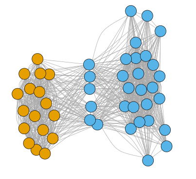
We clearly see that the two division cluster together with a lot of comparisons available between the teams. Six teams, those that got promoted and relegated between the two divisions, are clearly shown to fall in between the two large clusters. All comparisons to be made between teams in the two divisions has to rely on the information that is available via these six teams. Including all these teams in a Elo rating, starting with all ratings equal, will surely be completely wrong and will take some time to be realistic. All point exchange between the divisions will have to happen via the promoted and relegated teams.

I have previously investigated this in the context of regression models, where I demonstrated how including data from the Championship improves the prediction of Premier League matches. Se this and this.

So how can we find the initial ratings that will give realistic ratings that also calibrate the ratings between two or more leagues? By using a small amount of data, say one year worth of data, less that you would use to tune the K-factor and home field advantage, you can use an optimization algorithm to find the ratings that best fits the observed outcomes. In doing this you have to use the formula that converts the ratings to expected outcomes, but you do not use the update formula, so this approach can be seen as a static version of the Elo ratings.

Doing the direct optimization is however not completely straightforward. Elo ratings is a zero-sum system. No points are added or removed from the system, only exchanged. This constraint is similar to the sum-to-zero constraint that is sometimes used in regression modeling and Analysis-of-Variance. To overcome this, we can simply set the rating of one of the teams to the negative sum of the ratings of all the other teams.

A further refinement is to include home field advantage into the optimization. In cases where the teams have unequal number of home games, or some games where no teams play at home, this will create more accurate ratings. If not the ratings for those teams with an excess of home games will become unrealistically large.

Doing this procedure, using data from the Premier League and the Championship from 2010 which I used to make the graph above, I get the following ratings (with the average rating being 1500):

elo inits

The procedure also estimated the home field advantage to be 84.3 points.

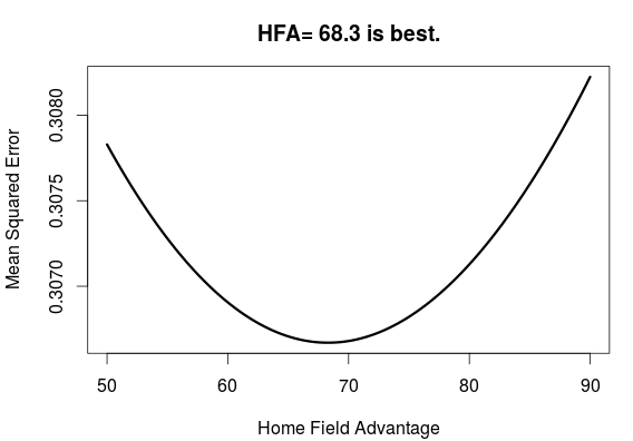
The data I used for the initial ratings is the first year of the data I used to tune the K-factor in the previous post. How does using these initial ratings influence the this tuning, compared with using the same initial rating for all teams? As expected, the optimal K-factor is smaller. The plot below shows that K=14 is the optimal K, compared with K=18.5 that I found last time. It is also interesting to see that the ratings with initialization are more accurate for the whole range of K’s I tested, than those without.

kwithinit

Tuning the Elo ratings: The K-factor and home field advantage

The Elo rating system is quite simple, and therefore easy implement. In football, FIFA uses is in its womens rankings and the well respected website fivethirtyeight.com also uses Elo ratings to make predictions for NBA and NFL games. Another cool Elo rating site is clubelo.com.

Three year ago I posted some R code for calculating Elo ratings. Its simplicity also makes it easy to modify and extend to include more realistic aspects of the games and competitions that you want to make ratings for, for example home field advantage. I suggest reading the detailed description of the clubelo ratings to get a feel of how the system can be modified to get improved ratings. I have also discussed some ways to extend the Elo ratings here on this blog as well.

If you implement your own variant of the Elo ratings it is necessary to tune the underlying parameters to make the ratings as accurate as possible. For example, a too small K-factor will give ratings that update too slow. The ratings will not adapt well to more recent developments. Vice versa, a too large K-factor will put too much weight on the most recent results. The same goes for the extra points added to the home team rating to account for the home field advantage. If this is poorly tuned, you will get poor predictions.

In order to tune the rating system, we need a way to measure how accurate the ratings are. Luckily the formulation of the Elo system itself can be used for this. The Elo system updates the ratings by looking at the difference between the actual results and the results predicted by the rating difference between the two opposing teams. This difference can be used to tune the parameters of the system. The smaller this difference is, the more accurate are the predictions, so we want to tune the parameters so that this difference is as small as possible.

To formulate this more formally, we use the following criterion to assess the model accuracy:

\( \sum_i[ (exp_{hi} – obs_{hi})^2 + (exp_{ai} – obs_{ai})^2 ] \)

where \(exp_{hi}\) and \(exp_{ai}\) are the expected results of match i for the home team and the away team, respectively. These expectations are a number between 0 and 1, and is calculated based on the ratings of the two teams. \(obs_{hi}\) and \(obs_{ai}\) are the actual result of match i, encoded as 0 for loss, 0.5 for draw and 1 for a win. This criterion is called the squared error, but we will use the mean squared error.

With this criterion in hand, we can try to find the best K-factor. Using data from the English premier league as an example I applied the ratings on the match results from the January 1st 2010 to the end of the 2014-15 season, a total of 2048 matches. I tried it with different values of the K-factor between 7 and 25, in 0.1 increments. Then plotting the average squared error against the K-factor we see that 18.5 is the best K-factor.

bestk185

The K-factor I have found here is, however, probably a bit too large. In this experiment I initialized the ratings for all teams to 1500. This includes the teams that was promoted from the Championship. A more realistic rating system would initialize these teams with a lower rating, perhaps be given the ratings from the relegated teams.

We can of course us this strategy to also find the best adjustment for the home field advantage. The simple way to add the home field advantage is to add some additional points to the ratings for the home team. Here I have used the same number of points in all matches across all season, but different strategies are possible. To find the optimal home field advantage I applied the Elo ratings with K=18.5, using different home field advantages.

besthfa683

From this plot we see that an additional 68.3 points is the optimal amount to add to the rating for the home team.

One might wonder if finding the best K-factor and home field advantage independent of each other is the best way to do it. When I tried to find the best K-factor with the home field advantage set to 68, I found that the best K was 19.5. This is a bit higher than when the home field advantage was 0. I tried to find the optimal pair of K and home field advantage by looking over a grid of possible values. Plotting the accuracy of the ratings against both K and the home field advantage in a contour we get the following:

besthfak

The best K and home field advantage pair can be read from the plot, both of which is a bit higher than the first values I found.

Doing the grid search can take a bit of time, especially if you don’t narrow down the search space by doing some initial tests beforehand. I haven’t really tried it out, but alternating between finding the best K-factor and home field advantage and using the optimal value from the previous round is probably going to be a reasonable strategy here.

My predictions for the 2016-17 Premier League

This year I am participating in Simon Gleave‘s Premier League prediction competition. It is an interesting initiative, as both statistical models and and more informal approaches are compared.

Last time I participated in something like this was midway trough the last Premier League season for statsbomb.com’s compilation. This time, however, the predictions are made before the first match has been played. To be honest, I think it is futile to try to model and predict an unplayed season since any model based only on previous results will necessarily reproduce what has already happened. This approach will work OK for predicting the result of the next couple of matches midway trough a season, but making predictions for the start of a season is really hard since the teams have brought inn some new players and gotten rid of other and perhaps also changed managers and so on. And not to forget that we also try predict results 9 months into the future.

When May comes and my predictions are completely wrong, I am not going to be embarrassed.

Last time I wanted to use the Conway-Maxwell-Poisson model, but I did not get it to work when I included data from several seasons plus data from the Championship. I still did not get it to work properly, but this time I tried a different approach to estimate the parameters. I ended up using a two-step approach, where I first estimate the attack and defense parameters with the independent Poisson model, and then, keeping those parameters fixed, I estimated the dispersion parameter by itself.

To fit the model I used Premier League data from the 2010-11 season to the 2015-16 season. I also included data from the 2015-16 season of the Championship (including the playoff) to be able to get some information on the promoted teams. I used the Dixon-Coles weighting scheme with \(\xi = 0.0019\). I used a separate parameter for home field advantage for Premier League and the Championship. I also used separate dispersion parameters for the two divisions.

I estimated the dispersion parameter for the Premier League to be 1.103, about the same as I previously estimated in some individual Premier League seasons, indicating some underdispersion in the goals. Interestingly, the dispersion parameter for the Championship was only 1.015.

Anyway, here are my projected league table with expected (or average) point totals. This is completely based on the model, I have not done any adjustments to it.

Team Points
Manchester City 73.70
Arsenal 69.73
Leicester City 64.12
Manchester United 63.95
Chelsea 63.84
Tottenham 62.53
Southampton 60.51
Liverpool 60.37
Everton 51.48
West Ham 51.12
Middlesbrough 46.30
Swansea 44.59
Burnley 44.20
Stoke City 42.99
Hull 42.49
Crystal Palace 41.33
Watford 41.23
Sunderland 39.83
West Bromwich Albion 39.21
Bournemouth 36.37