
One important characteristic of the Poisson distribution is that both its expectation and the variance equals parameter \(\lambda\). A consequence of this is that when we use the Poisson distribution, for example in a Poisson regression, we have to assume that the variance equals the expected value.
The equality assumption may of course not hold in practice and there are two ways in which this assumption can be wrong. Either the variance is less than the expectation or it is greater than the expectation. This is called under- and overdispersion, respectively. When the equality assumption holds, it is called equidispersion.
There are two main consequences if the assumption does not hold: The first is that standard errors of the parameter estimates, which are based on the Poisson, are wrong. This could lead to wrong conclusions when doing inference. The other consequence happens when you use the Poisson to make predictions, for example how many goals a football team will score. The probabilities assigned to each number of goals to be scored will be inaccurate.
(Under- and overdispersion should not be confused with heteroscedasticity in ordinary linear regression. Poisson regression models are naturally heteroscedastic because of the variance-expectation equality. Dispersion refers to what relationship there is between the variance and the expected value, in other words what form the heteroscedasticity takes.)
When it comes to modeling and predicting football results using the Poisson, a good thing would be if the data were actually underdispersed. That would mean that the probabilities for the predicted number of goals scored would be higher around the expectation, and it would be possible to make more precise predictions. The increase in precision would be greatest for the best teams. Even if the data were really overdispersed, we would still get probabilities that more accurately reflect the observed number of goals, although the predictions would be less precise.
This is the reason why I have looked into alternatives to the Poisson model that are suitable to model count data and that are capable of being over- and underdispersed. Except for the negative binomial model there seems to have been little focus on more flexible Poisson-like models in the literature, although there are a handful of papers from the last 15 years with some applied examples.
I should already mention the gamlss package, which is an extremely useful package that can fit a large number of regression type models in R. I like to think of it as the glm function on steroids. It can be used to create regression models for a large number of distributions (50+) and using different forms of dependent variables (for example random effects and splines) and doing regression on distribution parameters other than the usual expectation parameters.
The models that I have considered usually have two parameters. The two parameters are often not easy to interpret, but the distributions can be re-parameterized (which is done in the gamlss package) so that the parameters describe the location (denoted \(\mu\), often the same as the expectation) and shape (denoted \(\sigma\), often a dispersion parameter that modifies the association between the expectation and variance). Another typical property is that they equal the Poisson for certain values of the shape parameter.
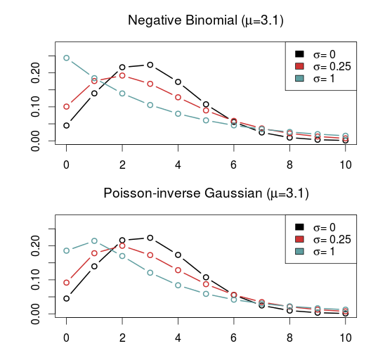
As I have already mentioned, the kind of model that is most often put forward as an alternative to the Poisson is the Negative binomial distribution (NBI). The advantages of the negative binomial are that is well studied and good software packages exists for using it. The shape parameter \(\sigma > 0\) determines the overdispersion (relative to the Poisson) so that the closer it is to 0, the more it resembles the Poisson. This is a disadvantage as it can not be used to model underdispersion (or equidispersion, although in practice it can come arbitrarily close to it). Another similar, but less studied, model is the Poisson-inverse Gaussian (PIG). It too has a parameter \(\sigma > 0\) that determines the overdispersion.
A large class of distributions, called Weighted Poisson distributions, is capable of being both over- and underdispersed. (The terms Weighted in the name comes from a technique used to derive the distribution formulas, not that the data is weighted) A paper describing this class can be found here. The general form of the probability distribution is
where \(t(x)\) is one of a large number of possible functions, and \(C(\theta,\alpha)\) is a normalizing constant which makes sure all probabilities in the distribution sum to 1. Note that I have denoted the two parameters using \(\theta\) and \(\alpha\) and not \(\mu\) and \(\sigma\) to indicate that these are not necessarily location and shape parameters. I think this and interesting class of distributions that I want to look more into, but since they are not generally implemented in any R package that I know of I will not consider them further now.
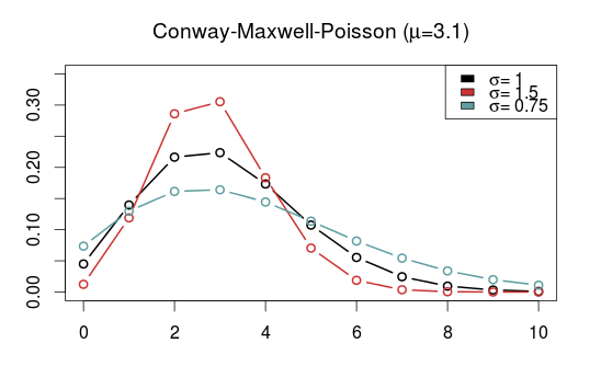
Another model that is capable of being over- and underdispersed is the Conway–Maxwell–Poisson distribution (COM), which incidentally is a special case of the class of Weighted Poisson distributions mentioned above (see this paper). The Poisson distribution is a special case of the COM when \(\sigma = 1\), and is underdispersed when \(\sigma > 1\) and overdispersed when \(\sigma\) is between 0 and 1. One drawback with the COM model is that the expected value depends on both parameters \(\mu\) and \(\sigma\), although it is dominated by \(\mu\). This makes the interpretation a bit difficult, but it may not be a problem when making predictions.
Unfortunately, the COM model is not supported by the gamlss package, but there are some other R packages that implements it. I have tried a few of them and the only one that I got to work is CompGLM, which for some reason does not use the location (\(\mu\)) and shape (\(\sigma\)) parameterization.
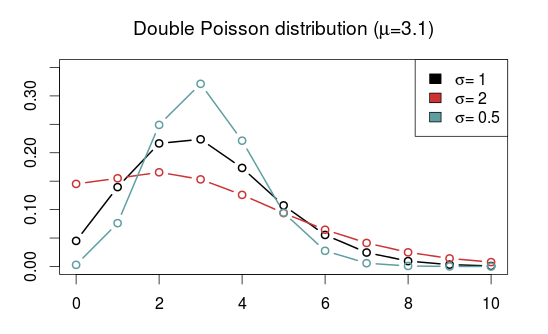
The Double Poisson (DP) is another interesting distribution which also equals the Poisson distribution when \(\sigma = 1\), but is overdispersed when \(\sigma > 1\) and underdispersed when \(\sigma\) is between 0 and 1. The expectation does not depend on the shape parameter \(\sigma\), and it is approximately equal to the location parameter \(\mu\). Another interesting thing about the Double Poisson is that it is belongs to a larger group of distributions called double exponential families which also lets you derive a binomial-like distribution with an extra dispersion parameter which can be useful in a logistic regression setting (see this paper, or this preprint).
In a follow up post I will try to use these distributions in regression models similar to the independent Poisson model.
